119. Equilibrium Search and Unemployment#
In addition to what’s in Anaconda, this lecture will need the following libraries:
!pip install quantecon
119.1. Overview#
This lecture studies Lucas and Prescott [1974], the labor-market companion to the paper on investment that we studied in Investment Under Uncertainty.
The two papers were written by the same authors at the same place within a few years of each other, and they use the same tools: a Bellman equation solved by successive approximations, Blackwell’s theorem, and a Markov process whose invariant distribution describes the long run.
What changes is the question.
Lucas and Prescott’s target was the natural rate of unemployment of Friedman [1968] and Phelps [1967].
In their words, the language used in discussing the natural rate “suggests that it may have the properties of a competitive equilibrium”, yet
there exist no theoretical models in which a nonzero equilibrium unemployment rate is determined and its properties studied.
Without such a model there was no framework in which to pose the welfare questions that unemployment raises, and no account of why average unemployment differs so much from one country to another.
The search literature of the 1960s could not supply one.
Job Search I: The McCall Search Model describes that literature’s central problem: a worker draws wage offers from a known distribution and decides when to stop searching.
It is a model of an individual, and it takes the wage distribution as given.
Lucas and Prescott argue that the questions they care about cannot be answered that way:
optimal labor supply behavior and the wage distribution on which it is based must be simultaneously determined within a model of market (as opposed to individual) behavior.
They build an economy of many spatially separate markets, each with its own randomly shifting demand for labor.
The picture comes from Edmund Phelps’s “island economy”, which they call “the direct ancestor of the present model” [Phelps and others, 1970].
It differs from the islands of Lucas [1972], where employment fluctuates with aggregate demand but unemployment, as an activity, is not distinguished from leisure.
Here it is distinguished.
Workers in a market can work at the wage that clears it, or leave.
Leaving means earning nothing this period and arriving somewhere else next period, so unemployment is the act of moving between markets.
Everything is competitive, everyone optimizes, and expectations are rational in the sense of Muth [1961] and of the investment paper, Lucas and Prescott [1971]: the distribution that workers use to evaluate their prospects is the one that their own decisions generate.
The paper’s central object is a single number, \(\lambda\), the expected present value of search.
An individual market takes \(\lambda\) as given, in the way a competitive firm takes a price as given.
Economy-wide, \(\lambda\) adjusts until the workforce that markets want to hold equals the workforce the economy has.
In the paper’s equilibrium some markets always have more workers than they want to employ, so unemployment is positive in every period; Three regions, one transition law explains when the computable version that we use keeps that property.
Lucas and Prescott also argue that this unemployment need not signal an inefficiency.
Note
There is no congestion externality in the model, and there is no matching function, no bargaining and no wage rigidity: unemployment is there because moving takes a period, and in equilibrium somebody is always moving.
The searching worker who crowds his fellows does so in the same way that any seller of a good crowds other sellers, and \(\lambda\), like any other equilibrium price, signals what the paper calls “the correct social return” to an additional searcher.
The paper proves no welfare theorem, and it leaves open whether actual labor markets have important external effects.
Efficiency shows that within the model the claim can be made exact: the stationary equilibrium maximizes the expected present value of surplus attainable from its own distribution of workers when moving takes a period, and \(\lambda\) is the present value of a worker added to the pool of searchers.
The lecture first sets out the theory: a worker’s problem, the two thresholds that describe a market, and the law of motion of a market’s workforce. It then computes an example, closes the economy by finding the equilibrium \(\lambda\), and asks how workers could learn it.
After a look inside the equilibrium, at markets, workforces and wages, it proves the efficiency claim and relates the model to its descendants. The exercises take up the paper’s comparative statics, a moving cost, the paper’s own two-state examples, undirected search, the Phillips curve, and a numerical check of efficiency.
Let’s start with some imports:
import warnings
import numpy as np
import matplotlib.pyplot as plt
import quantecon as qe
from collections import namedtuple
from scipy.optimize import brentq
119.2. The economy#
There are many markets, each with its own state of demand.
Demand shifts are independent across markets, so that aggregate demand is constant, and persistent within a market, so that today’s demand tells a worker something about tomorrow’s.
In each market a competitive industry produces a single good with labor as the only input.
If \(p = D(s, Q)\) is the inverse demand curve in demand state \(s\) and \(q(n)\) is the production function of each of the \(m\) identical firms, then profit maximization sets the wage equal to the marginal value product of labor, and the function
summarizes everything about the demand side of this labor market.
Lucas and Prescott discard \(D\) and \(q\) and place assumptions directly on \(R\): it is positive, bounded and differentiable, with
The demand state \(s\) follows a Markov process with transition density \(f(s', s)\) possessing a unique stationary distribution.
Its conditional distribution function \(F(s', s)\) is decreasing in \(s\), so that higher demand today makes higher demand tomorrow more likely.
119.2.1. Timing#
A market begins a period with a workforce \(y\), which is the most it can employ.
Then, within the period:
demand \(s\) is realized and the labor market clears, employing \(n \le y\) workers at the wage \(w = R(s, n)\)
the \(y - n\) workers who are not employed earn nothing and join the pool of searchers
employed workers remain in the market into next period; searchers are allocated across markets and arrive next period
So a worker is unemployed for exactly one period each time he moves, and the unemployed are workers in transit.
119.2.2. The value of search#
Because demand shifts are independent across markets and there are many of them, the economy-wide distribution of workers across markets is constant once it has settled down, even though each market’s workforce fluctuates.
A searcher’s prospects therefore do not depend on the market he is leaving, and the expected present value of search is a single number \(\lambda\).
Searchers are allocated to markets in a way that equalizes the expected value of arriving, so no market offers an arriving worker more than \(\lambda\).
We take \(\lambda\) as given for now and determine it in Economy-wide equilibrium.
119.3. A worker’s problem#
Let \(v(s, y, \lambda)\) be the expected present value of the earnings of a worker who finds himself in a market with demand \(s\) and workforce \(y\) at the start of a period, and let \(\beta \in (0,1)\) be the discount factor.
Lucas and Prescott arrive at a functional equation for \(v\) by considering three cases.
Case A: some workers leave. Departing workers get \(\lambda\). The workers who stay can have no more, since the leavers could have stayed, and no less, since they could have left. So \(v = \lambda\).
Case B1: all workers stay and no new workers arrive. Current employment is \(y\), the wage is \(R(s,y)\), and next period’s workforce is still \(y\):
Case B2: all workers stay and new workers arrive. Arriving workers are searchers, so the discounted expected value of being in this market next period, \(\beta \int v f\, ds'\), must be exactly \(\lambda\), the value of the search that brought them:
When the discounted continuation value at the unchanged workforce is below \(\lambda\), nobody arrives and case B1 applies; when it would exceed \(\lambda\), arrivals bring it down to \(\lambda\) and case B2 applies.
Either way the continuation is the smaller of \(\lambda\) and \(\beta \int v(s', y, \lambda) f(s', s)\, ds'\), which is the \(\min\) below.
Case A applies when even that leaves a worker with less than \(\lambda\), and then he takes \(\lambda\), which is the \(\max\).
All three cases collapse into one equation:
The two operators do different jobs. The max is the worker’s own option: he can always leave and collect \(\lambda\).
The min is not the worker’s choice at all. It is a restriction that competition among searchers imposes: if the continuation value in this market exceeded \(\lambda\), searchers would flow in until it did not.
Proposition 119.1
For each \(\lambda\), equation (119.2) has a unique bounded continuous solution \(v\), and successive approximations converge to it from any starting point.
The solution is nondecreasing in \(s\) and in \(\lambda\) and nonincreasing in \(y\).
The proof of Proposition 119.1 is the one used throughout Investment Under Uncertainty: the operator defined by the right side of (119.2) is monotone and satisfies a discounting condition, so Blackwell’s theorem [Blackwell, 1965] applies.
Monotonicity in \(s\) is where the assumption that \(F(s', s)\) decreases in \(s\) is used. A worker is worse off the more crowded his market, because a larger workforce means a lower marginal product and a lower wage, which is why \(v\) is nonincreasing in \(y\).
119.4. Employment, wages, and two thresholds#
With \(v\) in hand, the rest of a market’s behavior follows from two threshold rules.
119.4.1. How many work#
Let \(\bar n(s, \lambda)\) be the employment at which the marginal worker is just indifferent between staying and searching:
The left side is what a worker gets by staying when employment and next period’s workforce are both \(\bar n\): this period’s wage plus the discounted continuation. It is nonincreasing in \(\bar n\).
If marginal revenue reaches zero at some workforce, as it does in the computable version below, the value of being in a market that crowded has fallen to \(\lambda\), the left side is flat at \(\beta \lambda < \lambda\), and (119.3) cannot hold there.
On an integer workforce grid, (119.3) rarely holds with equality, and employment is the largest \(\bar n\) at which the left side is at least \(\lambda\).
Employment is then
and unemployment in this market is \(y - n\), which is positive exactly when the workforce exceeds \(\bar n\).
119.4.2. How many arrive#
A market attracts searchers only when it employs its whole workforce and the continuation value still exceeds \(\lambda\).
Let \(\bar y(s,\lambda)\) be the workforce at which that stops being true:
Arrivals fill a market up to \(\bar y(s, \lambda)\) and no further. Note that \(\bar y \le \bar n\), since \(R \ge 0\) means that any workforce whose continuation alone covers \(\lambda\) also covers it once the wage is added.
The inequality is strict wherever the marginal product is positive: a market just worth entering for a searcher is then strictly inside the range where everyone works.
In the worst demand state of the calibration below, both thresholds are zero at the equilibrium value of \(\lambda\), and the market employs nobody and attracts nobody.
119.4.3. Three regions, one transition law#
Together, (119.4) and (119.5) partition the \((s,y)\) plane into the three regions of the paper’s Figure 3:
region I, where \(y > \bar n(s, \lambda)\) and the market sheds workers down to \(\bar n(s,\lambda)\);
region II, between the two thresholds, where nobody moves;
region III, where \(y < \bar y(s, \lambda)\) and the market is filled up to \(\bar y(s,\lambda)\).
They give the law of motion for the workforce a very simple form:
The Bellman equation evaluates the continuation at the unchanged workforce \(y\), while the transition law moves the workforce somewhere else.
That is not an inconsistency, because the \(\max\) and the \(\min\) have already dealt with the two cases in which the workforce moves.
Where arrivals come, the \(\min\) replaces the continuation by \(\lambda\), and a market filled to \(\bar y\) is worth at least \(\lambda\) to anyone in it: exactly \(\lambda\) with a continuous workforce, and possibly a little more on the integer grid used below. Where workers leave, the \(\max\) replaces the whole expression by \(\lambda\).
The continuation at the unchanged \(y\) is therefore used only in the region where the workforce really is unchanged.
Note
The paper lets arrivals be random: a market short of workers receives \(a(s,y,\lambda)\,x\) of them, where \(x\) is a positive random variable with mean one, so that search must “eliminate rents on average” rather than exactly.
Like the numerical examples in the paper’s appendix, we set \(x \equiv 1\), which gives (119.6).
In the paper, random arrivals give the stationary distribution a strictly positive density (its Proposition 3), so some market is always shedding workers and unemployment is positive in every period.
With \(x \equiv 1\), finitely many demand states, and a demand process that can move between any two of them in one period, there are three cases.
If \(\max_s \bar y(s) > \min_s \bar n(s)\), the stationary distribution is unique and unemployment is positive: a market filled in the state with the highest \(\bar y\) sheds workers when demand falls to the state with the lowest \(\bar n\), and those two periods carry a market to \(\min_s \bar n(s)\) from any starting workforce.
If \(\max_s \bar y(s) = \min_s \bar n(s)\), the stationary distribution is again unique, every market holds that workforce, and unemployment is zero.
If \(\max_s \bar y(s) < \min_s \bar n(s)\), any workforce between the two stays where it is in every demand state, so there is a continuum of stationary distributions, and unemployment is zero.
Exercise 119.1 meets economies of the third kind.
119.5. A computable version#
We follow the appendix of Lucas and Prescott [1974]: a finite number of demand states, an integer workforce, and value function iteration on (119.2).
For the demand process we use the example in the paper’s footnote 7, in which \(\log s\) follows an AR(1) with persistence between zero and one.
We discretize it with seven states by Rouwenhorst’s method.
Unlike the method of Tauchen [1986], it matches the persistence and the stationary variance of \(\log s\) exactly, even when persistence is high; the solution to Exercise 119.1 shows what goes wrong otherwise.
For \(R\) we take a marginal revenue schedule that falls linearly in employment and reaches zero at a capacity \(N\),
With two demand states and \(N = 100\), this is the schedule of the paper’s Example 1, drawn in the top left panel of its Figure 5, scaled up by a factor of two.
The capacity is a departure from the theory, which assumes that \(R\) is positive everywhere, but it is one that the paper’s own examples make. It caps the workforce a market will ever want below \(N\), so the paper’s Proposition 5, which promises an equilibrium for every workforce per market, holds here only for workforces below that cap.
It also shapes how unemployment behaves when workers are plentiful, as we will see.
How steeply \(R\) falls sets how far employment moves when demand moves, and therefore how much there is to gain from sending a worker from one market to another; Exercise 119.3 takes that up.
The function make_model builds a market from any demand chain and marginal revenue schedule, and create_model builds the lecture’s economy with it.
Model = namedtuple('Model', ['P', 's', 'y', 'R', 'β'])

def linear_R(s, y, N=200):
    "Marginal revenue s (1 - n/N)^+, which reaches zero at the capacity N."
    return s[:, None]*np.maximum(1 - y[None, :]/N, 0.0)

def make_model(P, s, β=0.9, y_max=260, R=linear_R, **R_args):
    "A market with demand chain (P, s) and marginal revenue R on y = 0, ..., y_max."
    y = np.arange(y_max + 1)
    R_sy = R(s, y, **R_args)
    R_sy[:, 0] = 0.0                                # an empty market pays nothing
    return Model(P=P, s=s, y=y, R=R_sy, β=β)

def create_model(n_s=7, ρ=0.9, sd=0.26, β=0.9, N=200, y_max=260,
                 method='rouwenhorst'):
    """The island economy, with log demand an AR(1) discretized into n_s states.

    ρ and sd are the persistence and the stationary standard deviation of
    log demand, so that changing ρ alone does not change how variable
    demand is.  N is a market's capacity: marginal revenue reaches zero there.
    """
    σ = sd*np.sqrt(1 - ρ**2)
    if method == 'rouwenhorst':
        with warnings.catch_warnings():         # quantecon notes a change in its API
            warnings.filterwarnings('ignore', message='The API of rouwenhorst',
                                    category=UserWarning)
            mc = qe.markov.rouwenhorst(n_s, ρ, σ)
    else:
        mc = qe.markov.tauchen(n_s, ρ, σ)
    return make_model(mc.P, np.exp(mc.state_values), β, y_max, N=N)

model = create_model()
print("demand states:", model.s.round(3))
demand states: [0.529 0.654 0.809 1. 1.237 1.529 1.891]
The Bellman operator is (119.2) with the integral replaced by a sum.
Because the continuation is evaluated at the unchanged workforce, the equation is a separate problem for each \(y\), linked only across demand states, which is why it is cheap to solve and why the convention we adopt for an empty market affects nothing else.
We need some value of search to solve it, so we use \(\lambda = 7.1\) here, a value close to the equilibrium that Economy-wide equilibrium computes.
The argument c, a cost of leaving that is zero until Exercise 119.2, changes the worker’s outside option from \(\lambda\) to \(\lambda - c\).
def worker_value(model, λ, c=0.0, tol=1e-11, max_iter=10_000):
    "Solve the worker's functional equation; a worker who leaves collects λ - c."
    P, R, β = model.P, model.R, model.β
    v = np.full(R.shape, λ - c)
    for i in range(max_iter):
        v_new = np.maximum(λ - c, R + np.minimum(λ, β*(P @ v)))
        v_new[:, 0] = λ - c                         # an empty market holds no workers
        if np.max(np.abs(v_new - v)) < tol:
            return v_new, i
        v = v_new
    raise RuntimeError(f"no convergence in {max_iter} iterations at λ = {λ}")

v, iters = worker_value(model, 7.1)
print(f"converged in {iters} iterations")
converged in 105 iterations
The two thresholds are the largest employment, and the largest workforce, at which the relevant value still covers \(\lambda\).
def last_at_least(A, bar):
    "For each row of A, the largest index past 0 at which A ≥ bar, or 0 if none."
    return np.array([np.max(np.where(row >= bar)[0]) if (row[1:] >= bar).any() else 0
                     for row in A])

def thresholds(model, v, λ, c=0.0):
    "The employment threshold n̄(s) and the arrival threshold ȳ(s)."
    EV = model.β*(model.P @ v)                  # the continuation at an unchanged workforce
    n_bar = last_at_least(model.R + EV, λ - c)  # staying on as the marginal worker
    y_bar = last_at_least(EV, λ)                # ≤ n_bar, because R ≥ 0 and c ≥ 0
    return n_bar, y_bar

n_bar, y_bar = thresholds(model, v, 7.1)
print("n̄(s) =", n_bar)
print("ȳ(s) =", y_bar)
n̄(s) = [  0  16  45  69  90 109 124]
ȳ(s) = [ 0  0  3 33 58 79 97]
Employment is capped by \(\bar n\), arrivals fill up to \(\bar y\), and (119.6) moves the workforce.
The invariant distribution of that Markov chain on \((s, y)\) can be computed exactly.
One period of (119.6) either leaves a workforce where it is or carries it onto a threshold, so from a threshold the chain never leaves the set of thresholds, and we can solve the small chain on pairs \((s, t)\), with \(t\) running over the at most \(2 \times 7\) threshold values.
A workforce off the thresholds can carry probability in the long run only if it stays put in every demand state.
The ends of such an interval of workforces are themselves thresholds that stay put, so the chain on the thresholds then has more than one invariant distribution: that is the third case of the note in Three regions, one transition law.
So we let qe.MarkovChain find every invariant distribution of the small chain, and stop with an error, rather than pick one, when there is more than one.
The function also stops if a threshold reaches the top of the grid, where it would be cut off without warning.
class NotBracketed(ValueError):
    "A bisection was given a bracket that does not contain a switch."

class NotUnique(ValueError):
    "The invariant distribution of a market is not unique."

class GridTooSmall(ValueError):
    "A threshold has reached the top of the workforce grid."

def stationary_distribution(model, n_bar, y_bar):
    "The invariant distribution of the chain on (s, y), computed exactly."
    P, n_s = model.P, len(model.s)
    if n_bar.max() == model.y[-1]:
        raise GridTooSmall(f"n̄ reaches the top of the grid, y = {model.y[-1]}")
    T = np.unique(np.concatenate([n_bar, y_bar]))     # the threshold values
    k = len(T)
    Q = np.zeros((n_s*k, n_s*k))                       # the chain on (s, t), t in T
    for i in range(n_s):
        t_next = np.searchsorted(T, np.clip(T, y_bar[i], n_bar[i]))
        for j in range(k):
            Q[i*k + j, t_next[j]::k] = P[i]            # to (s', t_next[j]) for every s'
    ψ_T = qe.MarkovChain(Q).stationary_distributions
    if len(ψ_T) > 1:
        raise NotUnique(f"the chain on the thresholds has {len(ψ_T)} recurrent classes")
    ψ = np.zeros((n_s, len(model.y)))
    ψ[:, T] = ψ_T[0].reshape(n_s, k)
    return ψ

def market_outcomes(model, λ, c=0.0):
    "Everything about a market at a given value of search, when leaving costs c."
    v, _ = worker_value(model, λ, c)
    n_bar, y_bar = thresholds(model, v, λ, c)
    ψ = stationary_distribution(model, n_bar, y_bar)
    y = model.y[None, :]
    n = np.minimum(y, n_bar[:, None])                      # employment in each (s, y)
    w = np.take_along_axis(model.R, np.maximum(n, 1), axis=1)    # and the wage
    Φ = np.cumsum(model.R, axis=1)                         # surplus: see lps_efficiency
    employment, wage_bill = (ψ*n).sum(), (ψ*n*w).sum()
    return dict(v=v, n_bar=n_bar, y_bar=y_bar, ψ=ψ, n=n, w=w,
                workforce=(ψ*y).sum(), employment=employment,
                unemployment=(ψ*(y - n)).sum(),
                # the mean wage per employed worker; empty markets get no weight
                wage=wage_bill/employment if employment > 0 else np.nan,
                wage_bill=wage_bill,
                surplus=(ψ*np.take_along_axis(Φ, n, axis=1)).sum())

out = market_outcomes(model, 7.1)
print(f"workforce {out['workforce']:.2f}, employment {out['employment']:.2f}, "
      f"unemployment {out['unemployment']:.2f}")
workforce 49.92, employment 48.86, unemployment 1.06
The small chain has \(n_s |T|\) states, where \(|T| \le 2 n_s\) is the number of distinct thresholds, and finding its invariant distributions costs about \((n_s |T|)^3\) operations.
That is negligible with seven states and manageable with 25, where a whole equilibrium takes a second or two, but it becomes slow beyond about 35 states.
119.6. Economy-wide equilibrium#
So far \(\lambda\) has been a parameter.
Now close the model.
The economy has a fixed workforce, \(\mu\) per market.
For any \(\lambda\), the calculation above delivers the stationary distribution \(\Psi(s, y; \lambda)\) of a market’s demand and workforce, whose probabilities on our grid are the array ψ.
Averaging the workforce across markets with it gives the economy’s demand for workforce,
A higher \(\lambda\) makes every market shed workers sooner and fill up less, so \(E(y;\lambda)\) is decreasing.
Equilibrium is the \(\lambda^*\) at which markets want to hold exactly the workers the economy has:
Because the schedule is decreasing, bisection finds \(\lambda^*\).
On the integer grid \(E(y; \lambda)\) is a step function of \(\lambda\), which jumps whenever a threshold moves by one worker, so (119.8) holds only to within a step, and the workforces printed below and in the exercises differ slightly from \(\mu\).
equilibrium_λ first checks that \(\mu\) lies between the workforces demanded at the two ends of its bracket, and raises NotBracketed if it does not.
def workforce_demand(model, λ, c=0.0):
    "The average workforce per market at the value of search λ."
    return market_outcomes(model, λ, c)['workforce']

def bisect(test, lo, hi, tol=1e-4, checked=False):
    "Locate, to within tol, where a test that fails at lo and passes at hi switches."
    if not checked and (test(lo) or not test(hi)):
        raise NotBracketed(f"the test does not switch between {lo} and {hi}")
    while hi - lo > tol:
        mid = 0.5*(lo + hi)
        lo, hi = (lo, mid) if test(mid) else (mid, hi)
    return hi

def equilibrium_λ(model, μ, c=0.0, lo=0.01, hi=40.0):
    "Bisect on the decreasing demand schedule E(y; λ) = μ."
    E_lo, E_hi = workforce_demand(model, lo, c), workforce_demand(model, hi, c)
    if not E_lo > μ > E_hi:
        raise NotBracketed(f"μ = {μ} is not between E(y; {lo}) = {E_lo:.2f} "
                           f"and E(y; {hi}) = {E_hi:.2f}")
    return bisect(lambda λ: workforce_demand(model, λ, c) <= μ, lo, hi, checked=True)

μ = 50                        # workers per market, against a capacity of 200
λ_star = equilibrium_λ(model, μ)
eq = market_outcomes(model, λ_star)

print(f"equilibrium value of search  λ* = {λ_star:.3f}")
print(f"workforce per market            = {eq['workforce']:.2f}   (target {μ})")
print(f"employment per market           = {eq['employment']:.2f}")
print(f"unemployment per market         = {eq['unemployment']:.2f}")
print(f"unemployment rate               = {100*eq['unemployment']/eq['workforce']:.2f}%")
print(f"separation rate                 = "
      f"{100*eq['unemployment']/eq['employment']:.2f}% of the employed per period")
print(f"mean wage                       = {eq['wage']:.3f}")
equilibrium value of search  λ* = 7.096
workforce per market            = 49.94   (target 50)
employment per market           = 48.88
unemployment per market         = 1.06
unemployment rate               = 2.13%
separation rate                 = 2.18% of the employed per period
mean wage                       = 0.774
The capacity shows up in the bracket check.
Even at \(\lambda = 0.01\) a market wants no more than \(N - 1 = 199\) workers, so an economy with \(N = 200\) workers per market has no equilibrium, and equilibrium_λ says so instead of returning a number.
try:
    equilibrium_λ(model, 200)
except NotBracketed as err:
    print(err)
μ = 200 is not between E(y; 0.01) = 199.00 and E(y; 40.0) = 0.00
Lucas and Prescott draw the equilibrium as a demand curve meeting a vertical supply curve, which is exactly what it is.
grid = np.linspace(0.6, 15.0, 45)
demand = [market_outcomes(model, λ) for λ in grid]
E_y = np.array([d['workforce'] for d in demand])
E_u = np.array([d['unemployment'] for d in demand])

fig, axes = plt.subplots(1, 2, figsize=(11, 4))

axes[0].plot(E_y, grid, lw=2, label=r'demand $E(y;\lambda)$')
axes[0].axvline(μ, color='C1', lw=2, ls='--', label=r'supply $\mu$')
axes[0].plot(eq['workforce'], λ_star, 'ko', ms=8)
axes[0].set_xlabel('workforce per market')
axes[0].set_ylabel(r'value of search $\lambda$')
axes[0].legend()

axes[1].plot(E_y, E_u, lw=2)
axes[1].plot(eq['workforce'], eq['unemployment'], 'ko', ms=8)
axes[1].set_xlabel('workforce per market')
axes[1].set_ylabel('unemployment per market')
plt.tight_layout()
plt.show()
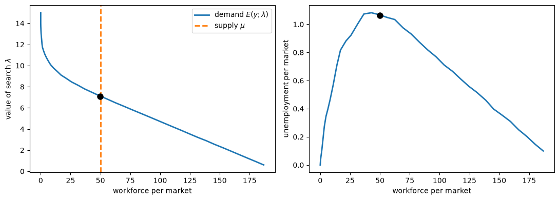
Fig. 119.1 The market for workers, and unemployment along the demand curve#
The left panel is the paper’s Figure 4. The right panel corresponds to the bottom panels of the paper’s Figure 5, which plot average unemployment against \(\lambda\) for two numerical examples; since \(E(y;\lambda)\) is decreasing, plotting it against the workforce instead shows the same hump, reflected.
Unemployment per market is not monotone in the size of the workforce, a feature that Lucas and Prescott report from their own examples, and the equilibrium sits near the top of the hump.
Where workers are abundant, \(\lambda\) is low, every market is pressed against its capacity, and the two thresholds of every demand state are squeezed together there, so even a large shift in demand moves few workers.
That side of the hump is the work of the capacity.
Where workers are scarce, \(\lambda\) is high, workforces are small, and many markets close altogether. Unemployment per market is small there only because there are so few workers per market; as a rate it is high, because the workers who remain are in the best markets and are shed whenever demand falls.
The unemployment rate and the share of empty markets both rise with \(\lambda\):
for λ in (0.6, λ_star, 10.0, 13.0):
    r = market_outcomes(model, λ)
    print(f"λ = {λ:6.3f}:  unemployment rate {100*r['unemployment']/r['workforce']:5.2f}%,"
          f"  markets with no workers {100*r['ψ'][:, 0].sum():5.1f}%")
λ =  0.600:  unemployment rate  0.05%,  markets with no workers   0.0%
λ =  7.096:  unemployment rate  2.13%,  markets with no workers   3.0%
λ = 10.000:  unemployment rate  5.56%,  markets with no workers  50.0%
λ = 13.000:  unemployment rate 12.02%,  markets with no workers  97.0%
119.7. Learning the value of search#
Lucas and Prescott devote a section of the paper to a question that the equilibrium itself does not answer: we have assumed that workers know \(\lambda\), and said nothing about how they would come to know it.
Ultimately, they write, this is “a question for psychological rather than economic theory, so we do not apologize for framing it here in ad hoc ‘adaptive’ terms”.
They also say why the question is manageable here. The distribution \(\Psi\) that workers must learn depends on their own behavior, so as their perceptions change, so does the thing they are learning, which “could, in general, raise insuperable analytical difficulties”.
It does not here, “since the only feature of \(\Psi\) which is relevant to worker decisions is the parameter \(\lambda\)”. That is the self-referential structure of Least Squares Learning in Self-Referential Models, collapsed to a single number.
Their answer is an adaptive story. Suppose workers believe the value of search is higher than it is; then more of them leave their markets than can be placed at that return.
In the paper the excess searchers are placed by letting the mean of the arrival variable \(x\) rise, so that receiving markets get more workers than they expected, and searchers and stayers alike are disappointed in the wages they expected. They revise the number down.
Writing \(g\) for a decreasing function that vanishes at zero,
Stability is built into the sign assumed for \(g\), and what justifies that sign is that the demand schedule slopes down: when \(\lambda\) is too high, markets want fewer workers than the economy has. equilibrium_λ rests on the same fact: it brackets the root rather than following the paper’s adjustment, but both work because \(E(y;\lambda)\) is decreasing.
The story can be put in discrete time: workers hold a belief \(\lambda_k\), markets act on it, and the belief is revised in the direction of the excess demand for workers,
This is Walrasian tâtonnement, with \(\lambda\) as the price and \(E(y;\lambda) - \mu\) as the excess demand. It has the form of the relaxation algorithm (91.3) of A Peculiar Definition of Bounded Rationality, applied to \(T(\lambda) = \lambda + E(y;\lambda) - \mu\), and the sign structure of E-stability: \(\lambda^*\) is stable because \(E(y;\lambda)\) slopes down.
The analogy is only formal, since \(T\) adds a number of workers to a present value and is not a map from a perceived to an actual value of \(\lambda\).
Near \(\lambda^*\) the error \(\lambda_k - \lambda^*\) is multiplied each step by \(1 + \gamma E'(\lambda^*)\), where \(E'\) is the slope of the schedule. So the iteration converges when \(0 < \gamma < 2/|E'(\lambda^*)|\), and converges without overshooting when \(\gamma < 1/|E'(\lambda^*)|\).
Because \(E(y;\lambda)\) is a step function on the integer grid, we estimate its slope by a centered difference wide enough to span many steps.
h = 0.5
slope = (workforce_demand(model, λ_star + h) - workforce_demand(model, λ_star - h))/(2*h)
print(f"slope of E(y; λ) near λ*: {slope:.1f}")
print(f"monotone convergence for γ < {1/abs(slope):.3f}, "
      f"convergence for γ < {2/abs(slope):.3f}")

def learn_λ(model, μ, γ, λ_0=10.0, n=40):
    "Revise the belief about λ in the direction of the excess demand for workers."
    path = [λ_0]
    for _ in range(n):
        path.append(path[-1] + γ*(workforce_demand(model, path[-1]) - μ))
    return np.array(path)

paths = {γ: learn_λ(model, μ, γ) for γ in (0.01, 0.05, 0.12)}
slope of E(y; λ) near λ*: -20.1
monotone convergence for γ < 0.050, convergence for γ < 0.100
Here are three gains, two below the bound and one above it.
fig, axes = plt.subplots(1, 2, figsize=(11, 4), sharey=True)
for ax, gains in zip(axes, ((0.01, 0.05), (0.12,))):
    for γ in gains:
        ax.plot(paths[γ], lw=2, label=fr'$\gamma = {γ}$')
    ax.axhline(λ_star, color='k', lw=0.8, ls='--', label=r'$\lambda^*$')
    ax.set_xlabel('iteration $k$')
    ax.legend(loc='upper right', framealpha=1)
axes[0].set_ylabel(r'belief $\lambda_k$')
plt.tight_layout()
plt.show()
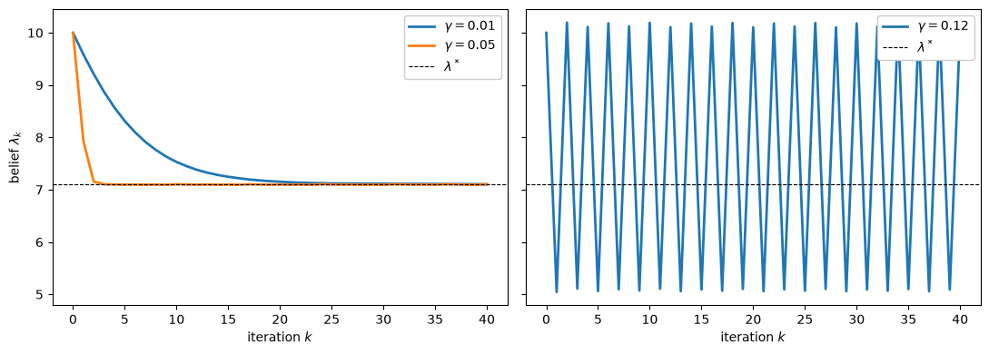
Fig. 119.2 Learning the value of search with gains below and above the bound#
With \(\gamma = 0.01\) the belief creeps down to \(\lambda^*\), and with \(\gamma = 0.05\), close to \(1/|E'|\), it gets there in a few steps.
With \(\gamma = 0.12\), above the bound, it does not converge: it jumps back and forth between a high and a low value, where the slope of the schedule is different and the overshooting stops growing.
The bounds are in units of value per worker: if every market were twice as large, \(E'\) would double and the stable gains would halve.
Lucas and Prescott are careful to add that this kind of stability “can have no relevance to the dynamic response to regularly recurring shocks”, which is the distinction between learning an equilibrium and responding within one. Least Squares Learning in Self-Referential Models studies what changes when agents estimate by least squares from data instead of evaluating \(E(y;\lambda)\) exactly.
119.8. Inside the equilibrium#
Now look inside the equilibrium: at a single market, at the distribution of workforces, and at the wages that identical workers are paid.
119.8.1. What a market looks like#
The thresholds describe the whole of a market’s behavior.
fig, axes = plt.subplots(1, 2, figsize=(11, 4))

axes[0].plot(model.s, eq['n_bar'], 'o-', lw=2, label=r'$\bar n(s)$: employment')
axes[0].plot(model.s, eq['y_bar'], 's--', lw=2, label=r'$\bar y(s)$: arrivals fill to')
axes[0].set_xlabel('demand state $s$')
axes[0].set_ylabel('workers')
axes[0].legend()

employs = eq['n_bar'] > 0                 # a state with n̄(s) = 0 employs nobody
wage_at_nbar = model.R[np.arange(len(model.s)), eq['n_bar']]
axes[1].plot(eq['n_bar'][employs], wage_at_nbar[employs], 'o-', lw=2)
axes[1].set_xlabel(r'employment $\bar n(s)$')
axes[1].set_ylabel('wage')
plt.tight_layout()
plt.show()
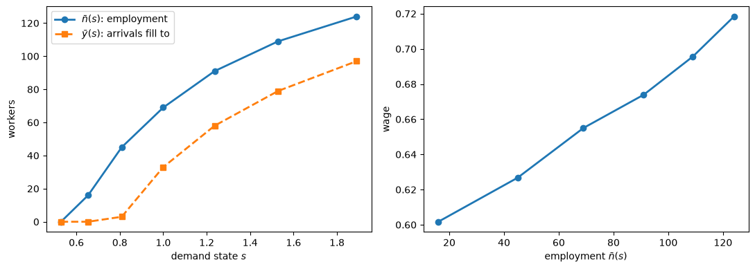
Fig. 119.3 The two thresholds at the equilibrium, and the locus of employment and wages as demand shifts#
The right panel is the curve that Lucas and Prescott call \(SS\), the pairs of employment and wages that a market would trace out as demand shifted if its workforce never constrained it.
It leaves out demand states with \(\bar n(s) = 0\), where a market employs nobody and pays no wage.
The curve is not flat. A flat \(SS\) would mean that workers had a single reservation wage, accepting work above it and searching below it, which is what the partial-equilibrium search model of Job Search I: The McCall Search Model derives.
At \(\bar n(s)\) the wage is whatever makes staying worth \(\lambda\), \(w = \lambda - \beta \int v(s', \bar n, \lambda) f(s', s)\, ds'\) up to the integer grid, so it moves opposite to the continuation value.
A fall in demand changes the continuation value in two ways that work in opposite directions:
lower demand today makes lower demand tomorrow more likely, which makes staying worth less;
lower employment today means a smaller workforce tomorrow, which makes staying worth more.
The first effect is present in partial-equilibrium models with persistent offers, such as Job Search VI: Persistent and Transitory Wage Shocks, where the reservation wage depends on the state.
The second comes from other workers’ decisions, and only an equilibrium model has it. Either can dominate, so \(SS\) can slope either way.
In this calibration it slopes upward, apart from small wiggles on finer grids among top demand states that markets almost never visit, so the second effect dominates: after a fall in demand, the continuation value in the smaller market is higher, and the wage that keeps its marginal worker is lower.
The equilibrium also shows the absence of a reservation wage directly.
ψ, n, w = eq['ψ'], eq['n'], eq['w']
sheds = model.y[None, :] > eq['n_bar'][:, None]          # region I: workers leave
occurs = (ψ > 1e-12) & (n > 0)                           # markets that occur and employ

print(f"lowest wage in a market that nobody leaves:  {w[occurs & ~sheds].min():.3f}")
print(f"highest wage in a market that workers leave: {w[occurs & sheds].max():.3f}")
lowest wage in a market that nobody leaves:  0.602
highest wage in a market that workers leave: 0.674
Workers stay on, and nobody leaves, in markets paying as little as the first number, while elsewhere workers walk away from markets paying the second, which is higher, so no cutoff between the two sorts the markets a worker accepts from those he leaves.
But the leavers are not turning down an offer in favor of something better, and nobody turns them away from it. At \(\bar n(s)\) every worker in the market, stayer or leaver, gets \(\lambda\); the leavers could stay, but then employment would be the whole workforce \(y\), the wage would fall to \(R(s, y)\), and staying would be worth less than \(\lambda\).
So no offer is rejected against a cutoff wage, and nobody is denied a job at the going wage: the margin is the market’s level of employment.
119.8.2. The workforce distribution and a sample path#
Because arrivals are deterministic and demand takes finitely many values, the workforce moves between a small number of values, each one a threshold of some demand state.
fig, axes = plt.subplots(1, 2, figsize=(12, 4))

ψ_y = eq['ψ'].sum(axis=0)                      # the distribution of the workforce
on_support = ψ_y > 1e-10
axes[0].stem(model.y[on_support], ψ_y[on_support], basefmt=' ')
axes[0].set_xlabel('workforce $y$')
axes[0].set_ylabel('probability')

T_path = 60
idx = qe.MarkovChain(model.P).simulate_indices(T_path, init=3, random_state=0)
path_y = np.empty(T_path, dtype=int)
path_y[0] = eq['n_bar'][idx[0]]
for t in range(T_path - 1):
    path_y[t+1] = np.clip(path_y[t], eq['y_bar'][idx[t]], eq['n_bar'][idx[t]])
path_n = np.minimum(path_y, eq['n_bar'][idx])

periods = np.arange(T_path)
axes[1].plot(periods, path_y, lw=2, drawstyle='steps-post', label='workforce')
axes[1].plot(periods, path_n, lw=2, ls='--', drawstyle='steps-post', label='employment')
axes[1].fill_between(periods, path_n, path_y, step='post', alpha=0.3, label='unemployed')
axes[1].set_xlabel('period')
axes[1].set_ylabel('workers')
axes[1].legend()
plt.tight_layout()
plt.show()

print(f"on this path demand falls {np.sum(idx[1:] < idx[:-1])} times, "
      f"and the market sheds workers in {np.sum(path_n < path_y)} periods")
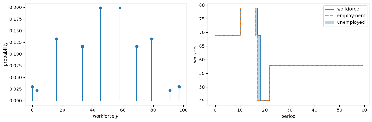
Fig. 119.4 The invariant distribution of the workforce, and one market over sixty periods#
on this path demand falls 7 times, and the market sheds workers in 2 periods
The right panel shows the mechanism of the model in one picture: a market is at rest whenever demand does not move.
When demand falls far enough that \(\bar n(s)\) drops below the workforce, the gap between the two lines opens, for that period only: that period’s leavers are the unemployed, and by the next period they are somewhere else.
A smaller fall need not open it: a market that was filled only to \(\bar y(s)\) can absorb a fall to a state whose \(\bar n\) is still above its workforce, and the printed counts show how often that happens on this path.
119.8.3. Where markets sit#
The three regions of (119.6) are a partition of the state space, so the invariant distribution says how much of the economy is in each.
def where_markets_sit(model, r):
    "Shares of markets in each region, and how often a market's demand stays put."
    y = model.y[None, :]
    sheds, fills = y > r['n_bar'][:, None], y < r['y_bar'][:, None]
    ψ, still = r['ψ'], ~sheds & ~fills
    return {'shedding workers': ψ[sheds].sum(), 'receiving workers': ψ[fills].sum(),
            'neither': ψ[still].sum(), 'with no workers': ψ[:, 0].sum(),
            'still, among the empty': ψ[still[:, 0], 0].sum()/ψ[:, 0].sum(),
            'demand stays put': ψ.sum(axis=1) @ np.diag(model.P)}

for name, share in where_markets_sit(model, eq).items():
    print(f"{name:>24}: {100*share:5.1f}%")
        shedding workers:   5.6%
       receiving workers:   5.6%
                 neither:  88.8%
         with no workers:   3.0%
  still, among the empty:  88.0%
        demand stays put:  75.0%
Most markets are completely still in any given period. A few percent shed workers, and all of the economy’s unemployment comes from those; about as many are taking workers in.
What must balance is the flow of workers, and it does: the workers leaving shedding markets are exactly the workers arriving in receiving ones, as Exercise 119.4 checks.
The fourth line counts markets that hold no workers at all, and the fifth shows that most of them are still.
Such a market emptied when demand fell to a state where \(\bar n(s) = 0\), and it stays empty while demand is too low for \(\bar y(s)\) to be positive; the rest are being refilled because demand has recovered.
These shares depend on the discretization. With seven demand states a market’s demand stays where it is three periods in four, as the last line shows; here are the same numbers with 25 states.
model_25 = create_model(n_s=25)
eq_25 = market_outcomes(model_25, equilibrium_λ(model_25, μ))
print(f"{'':>24}{'7 states':>10}{'25 states':>11}")
for (name, a), b in zip(where_markets_sit(model, eq).items(),
                        where_markets_sit(model_25, eq_25).values()):
    print(f"{name:>24}{100*a:>9.1f}%{100*b:>10.1f}%")
print(f"{'unemployment rate':>24}{100*eq['unemployment']/eq['workforce']:>9.2f}%"
      f"{100*eq_25['unemployment']/eq_25['workforce']:>10.2f}%")
                          7 states  25 states
        shedding workers      5.6%       8.2%
       receiving workers      5.6%       8.1%
                 neither     88.8%      83.7%
         with no workers      3.0%       4.0%
  still, among the empty     88.0%      91.9%
        demand stays put     75.0%      41.3%
       unemployment rate     2.13%      2.11%
With 25 states demand moves in more periods, by less each time, and somewhat more markets shed and receive workers, but most markets are still still and the unemployment rate is almost unchanged.
119.8.4. The wage distribution#
We can now return to the wage distribution, which the Overview said had to be determined together with the behavior of workers. The search literature hands its worker a distribution of wage offers and asks what he should do with it.
Here that distribution is an output: every market pays the marginal product of labor in it, and what a market pays depends on the demand it drew and on how many workers chose to be there.
weight = eq['ψ']*eq['n']                     # weight a market by the workers it employs
weight = weight/weight.sum()

w, p = eq['w'].ravel(), weight.ravel()
order = np.argsort(w)
w, p = w[order], p[order]
cdf = np.cumsum(p)
quantile = lambda q: w[np.searchsorted(cdf, q)]
mean = (w*p).sum()
flow = λ_star*(1 - model.β)                # the flow value of search

fig, ax = plt.subplots(figsize=(7.5, 4))
ax.hist(w, bins=30, weights=p, color='C0', alpha=0.85)
ax.axvline(mean, color='k', lw=1.5, label=f'mean {mean:.3f}')
ax.axvline(flow, color='C1', lw=1.5, ls='--', label=f'flow value of search {flow:.3f}')
ax.set_xlabel('wage')
ax.set_ylabel('share of workers')
ax.set_xlim(0.5, 1.45)            # a thin tail runs past this; see the print below
ax.legend()
plt.tight_layout()
plt.show()

print(f"mean {mean:.3f}, "
      f"p10 {quantile(0.1):.3f}, median {quantile(0.5):.3f}, p90 {quantile(0.9):.3f}")
print(f"p90/p10 = {quantile(0.9)/quantile(0.1):.2f},  "
      f"highest wage paid {w[p > 1e-12].max():.3f}")
print(f"share paid less than the flow value of search: {100*p[w < flow].sum():.0f}%")
near = np.abs(w - flow) < 0.001*flow
print(f"share paid within 0.1% of it: {100*p[near].sum():.1f}%")
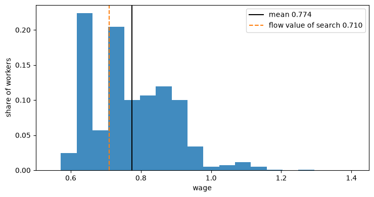
Fig. 119.5 Wages across identical workers, at the equilibrium#
mean 0.774, p10 0.627, median 0.748, p90 0.925
p90/p10 = 1.48,  highest wage paid 1.862
share paid less than the flow value of search: 31%
share paid within 0.1% of it: 9.2%
Workers in this economy are identical: they have the same skills, the same preferences and the same information, and they are free to leave at any time. They are nevertheless paid differently, by about half as much again at the ninetieth percentile as at the tenth.
The dispersion is not a market failure or a mistake. It is what equalizes the value of arriving in any market that takes workers, and of staying or leaving in any market that sheds them.
Everywhere else incumbents earn rents, because new workers take a period to arrive, so the values of positions are dispersed too.
held = eq['ψ']*model.y[None, :]              # weight a market by its workforce
print(f"λ* = {λ_star:.3f},  average value of a worker's position = "
      f"{(held*eq['v']).sum()/held.sum():.3f}")
print(f"share of workers whose position is worth more than λ*: "
      f"{100*held[eq['v'] > λ_star + 1e-9].sum()/held.sum():.0f}%")
λ* = 7.096,  average value of a worker's position = 7.548
share of workers whose position is worth more than λ*: 93%
About nine workers in ten hold a position worth more than \(\lambda^*\) to them.
The dashed line in the figure is the flow value of search, \((1-\beta)\lambda^*\), which is what a searcher’s position is worth per period.
Roughly a third of workers are paid less than that, and stay. The exact share is fragile.
On this grid a block of about one worker in eleven is paid within a tenth of a percent of the flow value, as the last line of the earlier print shows, so a small change in the grid can move the whole block across the line; across the grids we tried, the share runs from about 30 to 40 percent.
There is no puzzle in it: what a worker holds is not his current wage. It is a position in a particular market, which carries a claim on that market’s future and the option to walk away later.
119.9. Efficiency#
Lucas and Prescott say that \(\lambda\) signals “the correct social return from an additional unit supplied”, but they prove no welfare theorem.
The model has one, and its proof uses the device of the 1971 paper studied in Investment Under Uncertainty: find a planning problem that the equilibrium solves.
119.9.1. Surplus#
Write
for the area under the marginal revenue schedule up to employment \(n\).
By (119.1) it is the area under the inverse demand curve \(D(s, \cdot)\) up to the industry’s output, per firm: gross consumer surplus, the objective of the 1971 paper.
It equals the value of output only when the product price is given, \(D(s, Q) = s\), so we call it surplus.
119.9.2. A planner for one market#
Consider a planner who runs a single market and can move workers in and out of it, and who is credited \(\lambda\) for each worker it releases into the pool of searchers and charged \(\lambda\) for each worker it brings in.
If next period’s workforce is \(y'\), the planner employs \(\min\{y, y'\}\) workers this period and releases or brings in the difference, so its value satisfies
Here is the marginal-value argument. \(\Phi(s, \cdot)\) is concave because \(R\) falls with \(n\), so \(\Phi(s, \min\{y, y'\})\) is jointly concave in \((y, y')\), and maximizing over \(y'\) preserves concavity.
So \(W\) is concave in \(y\), and the planner’s choice is governed by marginal comparisons, made with the marginal value \(\Delta W(s, y) = W(s, y) - W(s, y-1)\).
Keeping one more worker into next period is worth his wage plus \(\beta \int \Delta W(s', y') f(s', s)\, ds'\), and releasing him is worth \(\lambda\); bringing one in costs \(\lambda\) and is worth the discounted continuation alone.
So the planner releases workers down to a threshold defined by (119.3) with \(\Delta W\) in place of \(v\), fills up to a threshold defined by (119.5) in the same way, and otherwise leaves the workforce alone.
Case by case, the marginal worker is worth \(\lambda\) where the planner releases, \(R + \lambda\) where it fills, since he saves the charge for one arrival, and \(R + \beta \int \Delta W f\, ds'\) in between.
These are cases A, B2 and B1, so \(\Delta W\) satisfies (119.2). By the uniqueness in Proposition 119.1, \(\Delta W = v\), so the planner’s thresholds are the equilibrium thresholds and its policy is (119.6).
Here is the aggregation argument. Give every market such a planner, with the same \(\lambda\), and add their objectives.
The terms \(\lambda (y_t - y_{t+1})\) add up to \(\lambda\) times the fall in the economy’s total workforce, because every worker released in one period arrives somewhere in the next.
For any feasible plan the total workforce is constant, so these terms add up to zero, and the sum of the planners’ objectives is the expected present value of surplus.
The equilibrium policy maximizes each planner’s objective, so it maximizes the sum. At \(\lambda = \lambda^*\) it is also feasible, because \(E(y; \lambda^*) = \mu\) keeps the total workforce constant.
So no feasible way of moving workers produces a higher expected present value of surplus than the stationary equilibrium.
119.9.3. What the theorem says, and what it does not#
Stated precisely, the stationary equilibrium maximizes the expected present value of surplus
starting from its own stationary distribution \(\Psi(\lambda^*)\),
among all feasible plans in which moving takes a period, including plans that are not stationary and plans that condition on other markets’ histories,
with a continuum of markets, so that the equilibrium plan keeps the economy’s workforce constant period by period,
up to the slack of the integer grid, on which \(E(y; \lambda^*)\) is within a step of \(\mu\) rather than equal to it.
\(\lambda^*\) is the present value of a worker added to the pool of searchers; per period, the multiplier on the constraint that the economy’s workforce is fixed is \((1-\beta)\lambda^*\), the flow value of search in the wage figure above.
The theorem is about total surplus, whoever receives it, and says nothing about how surplus is divided: Exercise 119.2 finds a policy that lowers surplus and still makes workers better off.
Nor does it rank steady states. Its comparison starts from \(\Psi(\lambda^*)\) and counts everything that happens along the way to any other allocation.
A policy that leads to a different steady state can raise surplus in that steady state while lowering the present value, because getting there costs surplus first.
Exercise 119.6 computes two examples, a small subsidy to moving and the thresholds of a planner more patient than the workers, and both raise steady-state surplus per worker above its equilibrium level.
This is the logic of the modified golden rule of growth theory, where a planner who discounts the future chooses less capital than the steady state that maximizes consumption, because building the extra capital costs consumption first.
Here reallocating a worker costs a period of his output now and pays off later, so a planner who discounts reallocates less, and has less unemployment, than one who maximizes steady-state surplus.
The efficiency is relative to the technology of moving, which takes a period, and the equilibrium has exactly as much unemployment as that technology makes worthwhile once the future is discounted at \(\beta\).
119.10. Relation to other lectures#
In the first footnote of Baley et al. [2023], there is no “standard model” of frictional unemployment but three workable classes of models: matching models in the Diamond-Mortensen-Pissarides tradition, equilibrium versions of McCall [1970], and search-island models in the tradition of Lucas and Prescott [1974].
Calibrated versions of all three fit data on labor market flows and deliver plausible responses of unemployment to policies like unemployment insurance and layoff taxes.
This lecture is the third class, and the McCall lectures in this series study the worker’s problem at the heart of the second, in partial equilibrium. What this model adds to them is everything on the other side of the offer.
The wage a worker is offered is the marginal product of labor in a market whose workforce was determined by where other workers decided to go, and the value of looking elsewhere, \(\lambda\), is the number that clears the economy-wide market for workers.
One consequence is that there is no reservation wage, as the \(SS\) curve showed. Another concerns the flow rates between employment and unemployment.
A Lake Model of Employment and Unemployment takes both rates as parameters: a job finding rate of \(0.283\) (which that lecture calls \(\lambda\), not to be confused with the value of search here) and a separation rate of \(0.013\) go in, and the unemployment rate comes out.
Lake Model with an Endogenous Job Finding Rate makes the job finding rate the outcome of a McCall problem, though still against a wage distribution that is given.
In this lecture the separation rate is an equilibrium object, while the job finding rate is essentially one by construction.
The separation rate printed above, around \(2.2\) percent of the employed per period, combines how often demand shifts carry a market below its employment threshold with how many workers each such market sheds.
Warning
The job finding rate in this model is essentially one.
A worker who leaves is placed in some market at the start of the next period, so a spell of unemployment lasts one period and the model has nothing to say about unemployment duration.
Strictly, a market that receives searchers can have its demand fall so far that it sheds more workers than it held before they arrived, so that some of the newcomers must move again; in this calibration that happens to fewer than one searcher in a hundred, even if newcomers are the first to go.
119.10.1. What the island model became#
Alvarez and Veracierto [1999] took this model and made it a tool for quantitative policy analysis, in their words by “modifying Lucas and Prescott’s (1974) island model to incorporate undirected search and out-of-the-labor-force participation”.
Four things change. Search becomes undirected: searchers “arrive uniformly across all islands”, so an island’s workforce next period is its own employment plus the same inflow every other island gets, whether it wants the workers or not.
A searcher can then land in a market that is itself shedding workers and have to move again, so the duration of unemployment becomes an equilibrium object; it averages \(2.4\) periods in their laissez-faire benchmark.
The nonemployed gain a second option, home production, so that labor force participation is a margin and the model has three states rather than two.
With home production the inflow of searchers is set by the indifference between searching and staying home, so the size of the labor force becomes an outcome, which matters because the policies they study act on whether people look for work at all.
Islands produce with a decreasing returns technology subject to persistent productivity shocks rather than facing a shifting demand curve. And agents trade a complete set of state-contingent securities.
Their laissez-faire equilibrium “is efficient (despite the search frictions)”, the analogue for their economy of Efficiency, and they use it as the benchmark for evaluating minimum wages, two models of unions, firing taxes and unemployment insurance, at a model period of six weeks.
A firing tax worth twelve months of average wages, for example, takes their unemployment rate down from \(5.3\) to \(3.7\) percent and pushes the average duration of unemployment up from \(2.4\) to \(5.1\) periods, while lowering welfare by \(2.1\) to \(2.3\) percent of consumption.
Note
Undirected search changes how \(\lambda\) is determined.
Under directed search \(\lambda\) is a price: raise it and every market sheds workers sooner and fills up less, so (119.8) pins it down as a market-clearing condition pins down any other price, and the \(\min\) in (119.2) makes every market that receives workers worth exactly \(\lambda\) to them.
Under undirected search a searcher lands in a market drawn at random, so \(\lambda\) needs a consistency condition of its own, and the common inflow \(U\) becomes a second unknown.
With a fixed population the model is still determinate: there are two conditions, the population and the consistency of \(\lambda\), for the two unknowns.
In this calibration the equilibrium exists and is unique once the inflow can be fractional, but uniqueness no longer follows, in general, from a single decreasing schedule.
Exercise 119.4 computes it: undirected search lowers the value of search, and it lowers unemployment too.
119.10.2. Returns to labor mobility#
Lucas and Prescott end their discussion of a moving cost with a conjecture, that “differences of this sort in the actual or perceived costs of changing jobs can help to account for the observed differences in average unemployment across occupations and among countries”.
Why average unemployment differs across countries became a central question for this class of models; Ljungqvist and Sargent [1998], for example, trace the rise of European unemployment to generous unemployment benefits interacting with a more turbulent economic environment.
Baley et al. [2025] call the returns to labor mobility, how much more a worker produces where he is going than where he is, “important intermediating forces in all modern macroeconomic models with frictional labour markets”.
Baley et al. [2023] show that the same quantity decides what a layoff tax does to unemployment, and whether skill losses at the time of a quit can reverse the effect of turbulence on unemployment. It is a property of the shock and of the technology that intermediates it, taken together.
Baley et al. [2025] find that calibrations to firm size dynamics, with shocks passed through neoclassical production functions, deliver returns to labor mobility that are robust to perturbations of parameters, while calibrations of per-worker productivity processes to labor market statistics can be fragile.
One of the models they study is that of Alvarez and Veracierto [2001], who calibrated a productivity process to the establishment data on job creation and destruction of Davis and Haltiwanger.
That paper is a different model from Alvarez and Veracierto [1999]: establishments hire at a common labor market whose location changes at random, wage contracts are rigid, and risk-averse agents without insurance markets self-insure and choose how hard to search.
An establishment produces \(z\, k^{\theta_k} n^{\theta_n}\) from capital \(k\) and labor \(n\), with productivity \(z\) and \(\theta_k + \theta_n < 1\).
Baley et al. [2025] streamline the model, dropping the cost of creating an establishment and a small firing tax, so that every establishment rents capital and hires labor in spot markets and they all equate marginal products, which gives
so a shock is amplified by an exponent that explodes as returns to scale approach one.
At Alvarez and Veracierto’s parameters, they find that a low-productivity establishment employs only \(3.81\) percent as many workers as a high-productivity one, a ratio of about \(26\), and that high-productivity establishments hold more than \(96\) percent of all employment: an exponent of about \(4.35\) turns a productivity ratio of \(2.12\) into an employment ratio of about \(26\).
That is a frictionless allocation, since every establishment hires in the same spot market. In the present model moving takes a period, and Exercise 119.3 asks how much of a ratio like \(26\) survives that friction, holding the technology and the shock like Alvarez and Veracierto’s.
119.11. Exercises#
Exercise 119.1
Lucas and Prescott [1974] report two comparative statics from their own numerical examples:
Overall, we found for low and high persistence in demand that unemployment rates were low. In the former case, there was little gained by reallocating workers, while in the latter reallocation occurred infrequently. As expected, the greater the variability of demand, holding the degree of persistence fixed, the greater the level of unemployment.
Check both in this calibration, holding \(\mu = 50\).
Compute the equilibrium unemployment rate for persistence \(\rho \in \{0.6, 0.8, 0.9, 0.95, 0.99\}\), holding the stationary standard deviation of \(\log s\) fixed at \(0.26\), and for stationary standard deviations \(\{0.10, 0.18, 0.26, 0.34, 0.45\}\), holding \(\rho = 0.9\). Explain the shapes you find.
With independent demand, \(\rho = 0\),
equilibrium_λstops with an error. Show that unemployment is then exactly zero and that the equilibrium \(\lambda\) is not unique. Why does this not contradict the paper’s Proposition 5, or its claim that unemployment is positive in every period?Repeat part 2 at \(\rho = 0.3\), first with seven demand states and then with 25. What does the comparison say about the low end of part 1?
Solution
Holding the stationary standard deviation fixed as \(\rho\) varies is what the argument sd of create_model already does, so each experiment is one call.
def u_rate(model, μ):
    "The equilibrium unemployment rate."
    r = market_outcomes(model, equilibrium_λ(model, μ))
    return r['unemployment']/r['workforce']

for ρ in (0.6, 0.8, 0.9, 0.95, 0.99):
    print(f"ρ = {ρ:<5}  unemployment rate {100*u_rate(create_model(ρ=ρ), μ):.2f}%")
print()
for sd in (0.10, 0.18, 0.26, 0.34, 0.45):
    print(f"sd = {sd:<5} unemployment rate {100*u_rate(create_model(sd=sd), μ):.2f}%")
ρ = 0.6    unemployment rate 0.86%
ρ = 0.8    unemployment rate 2.08%
ρ = 0.9    unemployment rate 2.13%
ρ = 0.95   unemployment rate 1.44%
ρ = 0.99   unemployment rate 0.50%
sd = 0.1   unemployment rate 0.22%
sd = 0.18  unemployment rate 0.97%
sd = 0.26  unemployment rate 2.13%
sd = 0.34  unemployment rate 3.13%
sd = 0.45  unemployment rate 3.89%
Variability does what one expects: demand that moves further moves more workers, and the unemployment rate rises steadily with it.
Persistence does not: unemployment rises to a peak at \(\rho\) around \(0.8\) to \(0.9\), and falls again to about a quarter of the peak at \(\rho = 0.99\). That is the shape Lucas and Prescott describe, and the two ends are low for different reasons.
When demand is nearly independent across periods, a market that is unlucky today expects to be average tomorrow, so the value of staying hardly depends on today’s demand, the arrival threshold \(\bar y(s)\) barely varies with \(s\), and few workers are ever shed; part 2 takes this to its limit.
When demand is nearly permanent, it changes little from one period to the next: on the seven-state chain it changes rarely, by a whole notch, and on finer chains more often, by less. Either way few workers have reason to move in any one period, which is the paper’s “reallocation occurred infrequently”.
Unemployment needs demand shifts that are both worth responding to and frequent, a combination that only intermediate persistence delivers.
For part 2, equilibrium_λ stops because the invariant distribution is not unique, the third case of the note in Three regions, one transition law. So we look instead for the values of \(\lambda\) at which a market holding \(\mu\) workers never moves, \(\max_s \bar y(s) \le \mu \le \min_s \bar n(s)\).
Both thresholds fall as \(\lambda\) rises, so each end of that set is found by bisection.
def rest_interval(model, μ, lo=0.01, hi=40.0):
    "The interval of λ at which a market holding μ workers never moves, or None."
    def ends(λ):
        n_bar, y_bar = thresholds(model, worker_value(model, λ)[0], λ)
        return y_bar.max(), n_bar.min()
    λ_a = bisect(lambda λ: ends(λ)[0] <= μ, lo, hi)     # no market fills past μ
    λ_b = bisect(lambda λ: ends(λ)[1] < μ, lo, hi)      # some market sheds below μ
    return (λ_a, λ_b) if λ_a < λ_b else None

m_iid = create_model(ρ=0.0)
n_bar_iid, y_bar_iid = thresholds(m_iid, worker_value(m_iid, 7.1)[0], 7.1)
print("rows of P identical:", np.allclose(m_iid.P, m_iid.P[0]))
print("at λ = 7.1:  n̄(s) =", n_bar_iid, "  ȳ(s) =", y_bar_iid)
print("λ at which a market holding μ never moves: from {:.3f} to {:.3f}".format(
      *rest_interval(m_iid, μ)))
rows of P identical: True
at λ = 7.1:  n̄(s) = [ 55  57  61  71  88 107 124]   ȳ(s) = [47 47 47 47 47 47 47]
λ at which a market holding μ never moves: from 6.935 to 7.378
With independent demand every row of \(P\) is the same, so the continuation \(\beta \sum_{s'} v(s', y) P(s, s')\) does not depend on \(s\), and neither does \(\bar y\).
Since \(\bar y(s) \le \bar n(s)\) in every state, the common \(\bar y\) lies below every employment threshold. So every workforce between \(\bar y\) and \(\min_s \bar n(s)\) stays where it is in every demand state, markets drift into that interval and stop, and in the long run nobody moves and unemployment is exactly zero.
Every workforce in the interval is absorbing, so the invariant distribution is not unique, and every \(\lambda\) in the printed interval supports an equilibrium in which every market holds \(\mu\) workers.
The width of the interval is a property of the discretized chain: it narrows as states are added, because the worst demand state moves further out and its employment threshold comes down toward the common \(\bar y\). Unemployment stays at zero, though, since every \(\bar n(s)\) is at least \(\bar y\).
None of this contradicts the paper, and the operative difference is \(x \equiv 1\). The unique \(\lambda\) of Proposition 5 and the claim that unemployment is positive in every period both rest on the unique stationary density of Proposition 3, which random arrivals deliver by overfilling some markets, and with deterministic arrivals that argument is not available.
Independent demand also violates the strict monotonicity of \(F(s', s)\) in \(s\) that the paper maintains, and the example in its footnote 7 requires the AR(1) coefficient to be strictly positive.
For part 3, the same check at \(\rho = 0.3\) gives different answers on the two grids.
for n_s in (7, 25):
    m = create_model(n_s=n_s, ρ=0.3)
    rest = rest_interval(m, μ)
    if rest is not None:
        print(f"{n_s:>2} states: at rest for λ from {rest[0]:.3f} to {rest[1]:.3f}")
    else:
        print(f"{n_s:>2} states: unique λ*, unemployment rate {100*u_rate(m, μ):.3f}%")
 7 states: at rest for λ from 7.128 to 7.207
25 states: unique λ*, unemployment rate 0.014%
With seven states, persistence of \(0.3\) is not enough to spread the arrival thresholds past the lowest employment threshold, and the economy is at rest, as at \(\rho = 0\). With 25 states the extreme demand states are further out, the equilibrium is unique, and unemployment is positive but tiny.
So at \(\rho = 0.3\) unemployment is low on either grid, as the paper says, but whether it is exactly zero is a property of the discretized chain.
The method of discretizing matters more at the other end.
def chain_moments(m):
    "Standard deviation and autocorrelation of log s, and the chance that s stays put."
    π = qe.MarkovChain(m.P).stationary_distributions[0]
    x = np.log(m.s) - π @ np.log(m.s)
    sd = np.sqrt(π @ x**2)
    return sd, (π*x) @ (m.P @ x)/sd**2, π @ np.diag(m.P)

print(f"{'method':>12}{'ρ':>6}{'sd':>8}{'autocorr':>10}{'P(stay)':>9}{'u rate':>9}")
for ρ in (0.9, 0.99):
    for method in ('rouwenhorst', 'tauchen'):
        m = create_model(ρ=ρ, method=method)
        sd, ac, stay = chain_moments(m)
        print(f"{method:>12}{ρ:>6}{sd:>8.3f}{ac:>10.4f}{stay:>9.3f}"
              f"{100*u_rate(m, μ):>8.2f}%")
      method     ρ      sd  autocorr  P(stay)   u rate
 rouwenhorst   0.9   0.260    0.9000    0.750    2.13%
     tauchen   0.9   0.304    0.9016    0.733    2.68%
 rouwenhorst  0.99   0.260    0.9900    0.971    0.50%
     tauchen  0.99   0.343    0.9999    1.000    0.01%
Rouwenhorst’s chain has exactly the target standard deviation, \(0.26\), and the target autocorrelation. Tauchen’s seven-state chain is too volatile at \(\rho = 0.9\), which raises unemployment by about a quarter.
At \(\rho = 0.99\) it is too volatile and also far too persistent: its demand state almost never changes, so markets almost never reallocate, and unemployment nearly vanishes.
With seven states, that would make the right end of part 1 look like the left; with 25 states the two methods nearly agree.
Exercise 119.2
In their concluding section, Lucas and Prescott consider a lump-sum cost \(c\) of leaving a market to search, so that the right side of (119.3) becomes \(\lambda - c\) rather than \(\lambda\): a worker who leaves collects the value of search net of what it costs him to get there.
The arrival condition (119.5) is unchanged, since it prices the market for workers who are already searching.
They say that the cost “will raise the curve \(y = \bar n(s, \lambda)\) in Fig. 3 and shift the ‘demand curve’ in Fig. 4 downward. The result is a decrease in unemployment and a decrease in the equilibrium present value of wages, \(\lambda\)”, and remark that this
shows that lower average unemployment is not, in general, associated with higher welfare for workers.
market_outcomes and equilibrium_λ already take the cost as their argument c.
For \(c \in \{0, 0.2, 0.5, 1, 2\}\) report the equilibrium \(\lambda^*\) and \(\lambda^* - c\), the unemployment rate, surplus per market, the wage bill per market, rents (surplus minus the wage bill), and workers’ income per worker per period, the wage bill net of what workers pay to move, divided by the workforce.
Does \(\lambda^*\) fall, as the paper says? If not, what does?
Does lower unemployment mean better off? Compare what workers gain with what the economy loses, as present values per worker.
Who pays? Answer once treating \(c\) as a resource, used up in moving, and once treating it as a tax whose revenue is rebated lump sum to workers.
Baley et al. [2023] use the smallest layoff tax that shuts down all endogenous separations as a diagnostic of a model’s returns to labor mobility. Compute the smallest \(c\) that does that here, in units of the average wage, with 7, 15 and 25 demand states. Why does it change with the number of states?
Solution
Before sweeping, look at what the cost does to workforce demand at the laissez-faire value of search.
λ_0 = equilibrium_λ(model, μ)
for c in (0.0, 2.0):
    n_bar_c, y_bar_c = thresholds(model, worker_value(model, λ_0, c)[0], λ_0, c)
    print(f"c = {c}: workforce demand {workforce_demand(model, λ_0, c):5.1f},  "
          f"n̄(s) = {n_bar_c},  ȳ(s) = {y_bar_c}")
c = 0.0: workforce demand  49.9,  n̄(s) = [  0  16  45  69  91 109 124],  ȳ(s) = [ 0  0  3 33 58 79 97]
c = 2.0: workforce demand  74.8,  n̄(s) = [ 62  78  93 107 121 134 146],  ȳ(s) = [ 0  0  2 31 54 72 87]
The cost raises workforce demand, so the new \(\lambda^*\) lies above the old one, and we start each bisection there. That also keeps it away from low values of \(\lambda\), where with a cost the invariant distribution is not unique and the bisection would stop.
In a stationary distribution every unemployed worker left his market once this period, so workers pay \(c\) times unemployment per market in moving costs.
results = {}
for c in (0.0, 0.2, 0.5, 1.0, 2.0):
    λ_c = equilibrium_λ(model, μ, c, lo=λ_0) if c > 0 else λ_0
    results[c] = (λ_c, market_outcomes(model, λ_c, c))

income = lambda r, c: (r['wage_bill'] - c*r['unemployment'])/r['workforce']
rents = lambda r: r['surplus'] - r['wage_bill']

print(f"{'c':>5}{'λ*':>8}{'λ*-c':>8}{'u rate':>9}{'surplus':>9}{'wages':>8}"
      f"{'rents':>8}{'income':>9}")
for c, (λ_c, r) in results.items():
    print(f"{c:>5}{λ_c:>8.3f}{λ_c - c:>8.3f}"
          f"{100*r['unemployment']/r['workforce']:>8.2f}%{r['surplus']:>9.3f}"
          f"{r['wage_bill']:>8.3f}{rents(r):>8.3f}{income(r, c):>9.4f}")
    c      λ*    λ*-c   u rate  surplus   wages   rents   income
  0.0   7.096   7.096    2.13%   46.708  37.844   8.864   0.7577
  0.2   7.206   7.006    1.65%   46.586  37.987   8.600   0.7575
  0.5   7.371   6.871    1.21%   46.351  38.167   8.184   0.7601
  1.0   7.661   6.661    0.73%   46.134  38.464   7.671   0.7625
  2.0   8.262   6.262    0.24%   45.325  38.434   6.892   0.7684
Surplus, wages and rents are flows per market, and income is a flow per worker. To compare what workers gain with what the economy loses, put both in present values per worker, dividing flows per worker by \(1 - \beta\).
β = model.β
r_0 = results[0.0][1]
pv = lambda flow: flow/(1 - β)
surplus_pw = lambda r: r['surplus']/r['workforce']
print(f"{'c':>5}{'workers gain':>14}{'surplus lost':>14}{'ratio':>7}")
for c, (_, r) in results.items():
    gain = pv(income(r, c) - income(r_0, 0.0))
    loss = pv(surplus_pw(r_0) - surplus_pw(r))
    ratio = f"{loss/gain:7.1f}" if gain > 0 else f"{'':>7}"
    print(f"{c:>5}{gain:>14.4f}{loss:>14.4f}{ratio}")

r_2 = results[2.0][1]
print(f"\nc = 2: unemployment falls {100*(1 - r_2['unemployment']/r_0['unemployment']):.0f}%, "
      f"the wage bill rises {100*(r_2['wage_bill']/r_0['wage_bill'] - 1):.1f}%, "
      f"rents fall {100*(1 - rents(r_2)/rents(r_0)):.0f}%")
print(f"moving costs paid, a present value per worker: "
      f"{pv(2.0*r_2['unemployment']/r_2['workforce']):.4f}")
    c  workers gain  surplus lost  ratio
  0.0        0.0000        0.0000
  0.2       -0.0020        0.0214
  0.5        0.0239        0.0473    2.0
  1.0        0.0480        0.1181    2.5
  2.0        0.1068        0.2344    2.2

c = 2: unemployment falls 89%, the wage bill rises 1.6%, rents fall 22%
moving costs paid, a present value per worker: 0.0472
For part 1, Lucas and Prescott say that the cost shifts the demand curve of their Figure 4 down and lowers \(\lambda\), but here it does the opposite.
At the laissez-faire \(\lambda^*\), the cost raises workforce demand by about half. It raises the employment threshold \(\bar n(s)\) in every state where anyone works, by a lot, since a worker who would leave now gives up \(c\) as well, while it lowers the arrival thresholds a little.
That is the paper’s own first step, “raise the curve \(y = \bar n(s, \lambda)\)”, and with \(\lambda\) on the vertical axis of Figure 4 it shifts the demand curve up, not down.
With more workers wanted than the economy has, \(\lambda^*\) must rise, and it does. What falls is \(\lambda^* - c\), the value of the option to leave net of its cost, which is what a worker deciding whether to stay compares with staying, and the paper’s statement holds for that number, not for \(\lambda^*\) itself.
For part 2, a cost of two cuts measured unemployment by close to nine tenths. Measured by their income net of moving costs, workers gain clearly from \(c = 0.5\) on.
For smaller costs what they pay to move nearly offsets the extra wages, so the gain is close to zero, and on this grid it is slightly negative at \(c = 0.2\).
The economy loses more than workers gain: at \(c = 2\) surplus falls by about two to two and a half times as much as workers’ income rises. These are comparisons of steady states, which leave out the transition from one to the other.
So lower unemployment is not a welfare index, but the lesson arrives in a different form from the paper’s: Lucas and Prescott’s workers are worse off because \(\lambda\) falls, while ours are better off and the economy as a whole is worse off.
The unemployment that the cost eliminated was productive. Those workers were not idle in any useful sense; they were in transit from markets where their marginal product had fallen to markets where it was high, and the cost keeps them where they are.
For part 3, the wage bill rises a little, while rents, surplus minus the wage bill, fall by about a fifth.
Surplus is the area under \(R\), so rents are the profits of firms plus, when product demand slopes down, the consumer surplus of the buyers of the market’s good, and it is they who pay.
How the account closes depends on what \(c\) is. If it is a real resource, the moving costs printed above are used up as well, on top of the lost surplus, and workers bear them.
If it is a tax rebated lump sum to workers, nothing is used up beyond the lost surplus, and the rebate returns those same moving costs to workers each period without changing anyone’s decisions, so workers gain more.
The two cases differ in what the lost surplus means, too. Exercise 119.6 shows that with a resource cost the equilibrium is the planner’s allocation for the costlier technology of moving, so the lower surplus is the price of a worse technology, not an inefficiency; with a rebated tax the technology is unchanged and the equilibrium is no longer the planner’s allocation for it, so the lower surplus is an efficiency loss.
For part 4, recall the note in Three regions, one transition law. Separations stop exactly when there is a \(\lambda\) at which a market holding \(\mu\) workers never moves, with no state’s arrival threshold above \(\mu\) and no state’s employment threshold below it.
A cost raises the employment thresholds, so we look for the smallest cost at which such a \(\lambda\) exists.
Once separations stop every market holds \(\mu\) workers for ever, so a worker in demand state \(s\) holds \(v_s\), with \(v = (I - \beta P)^{-1} R(\cdot, \mu)\), and nobody leaves or arrives when \(\beta (Pv)_s \le \lambda \le v_s + c\) for every \(s\).
That gives a formula to set beside the computation, \(c_{\min} \approx \beta \max_s (Pv)_s - \min_s v_s\), which ignores the integer grid.
def at_rest_values(model, μ):
    "The value of a position when every market holds μ workers for ever."
    return np.linalg.solve(np.eye(len(model.s)) - model.β*model.P, model.R[:, μ])

def min_cost(model, μ, lo=1.0, hi=20.0, c_hi=20.0):
    "The smallest c at which some λ leaves a market holding μ workers at rest."
    def at_rest(c):
        ends = lambda λ: thresholds(model, worker_value(model, λ, c)[0], λ, c)
        λ_a = bisect(lambda λ: ends(λ)[1].max() <= μ, lo, hi, tol=1e-3)  # nobody fills past μ
        n_bar, y_bar = ends(λ_a)
        return y_bar.max() <= μ <= n_bar.min()
    return bisect(at_rest, 0.0, c_hi, tol=1e-2)

print(f"{'states':>7}{'c_min/wage':>12}{'formula':>9}{'log s ranges over':>20}")
for n_s in (7, 15, 25):
    m = create_model(n_s=n_s)
    v_rest = at_rest_values(m, μ)
    wage = qe.MarkovChain(m.P).stationary_distributions[0] @ m.R[:, μ]
    formula = m.β*(m.P @ v_rest).max() - v_rest.min()
    print(f"{n_s:>7}{min_cost(m, μ)/wage:>12.2f}{formula/wage:>9.2f}"
          f"{np.log(m.s).min():>11.2f} to {np.log(m.s).max():.2f}")
 states  c_min/wage  formula   log s ranges over
      7        4.91     4.99      -0.64 to 0.64
     15        8.30     8.39      -0.97 to 0.97
     25       11.67    11.77      -1.27 to 1.27
The wage used as the unit is the average wage when every market holds \(\mu\) workers, which is what the economy looks like once separations stop; it is within half a percent of the laissez-faire average wage.
The cost that stops all separations grows with the number of states, and the formula says why. It is set by the gap between the best and the worst demand state a market can be in, and Rouwenhorst’s chain places its extreme states at \(\pm 0.26 \sqrt{n_s - 1}\) in \(\log s\), so they move apart as states are added.
\(\log s\) itself is an AR(1) with unbounded support, so for the model with continuous demand no finite cost stops all separations: the number computed here measures the support of the discretized demand process.
For the symmetric two-state chain of Exercise 119.3, in which demand stays put with probability \(\rho\) and \(R(s,n) = s\, g(n)\), the formula has a closed form,
about \(1.05\) periods’ wages there, which depends on the demand process and \(\beta\) but not on the shape of \(g\): in this model the diagnostic measures the spread and persistence of demand, not the curvature of \(R\).
The calibration does not say how long a period is; with \(\beta = 0.9\) it is naturally read as a year, which would make every spell of unemployment a year long. For comparison, in the Ljungqvist–Sargent matching model that Baley et al. [2023] use as their benchmark, layoff taxes of \(163\) to \(184\) percent of a year’s output per worker shut down all endogenous separations, at a model period of half a quarter.
Baley, Ljungqvist and Sargent’s point is that this number has to be large to be credible, because extensive reallocation is observed in economies whose layoff costs differ enormously.
Exercise 119.3
The numerical examples in the appendix of Lucas and Prescott [1974] use just two demand states, with
Here \(\rho\) is the probability that demand stays where it is, so the autocorrelation of \(s\) is \(2\rho - 1 = 0.8\); in the seven-state chain \(\rho\) is the autocorrelation itself.
Build that economy, keeping \(R(s,n) = s\,(1 - n/N)^{+}\) with \(N = 200\), and \(\mu = 50\) wherever an equilibrium is needed.
For \(\lambda\) on a grid, plot workforce demand and average unemployment against \(\lambda\), as in the middle and bottom panels of the paper’s Figure 5.
At \(\lambda = 6\), show that the invariant distribution puts all of its mass on two values of the workforce, and say which two.
Use that fact to derive a formula for average unemployment per market in terms of \(\bar n\), \(\bar y\) and \(\rho\), check it against the computed value at every \(\lambda\) on the grid, and use it to explain the shape of the plot in part 1.
Show that the unemployment rate depends only on \(\rho\) and on \(r = \bar y(s_{\text{high}})/\bar n(s_{\text{low}})\), and that it can never exceed \(1 - \rho\).
Now replace \(R\) by the marginal product of a decreasing returns technology: output \(s\, n^{\alpha}\) with \(0 < \alpha < 1\), so that \(R(s, n) = s\,\alpha\, n^{\alpha-1}\). Solve for \(\alpha \in \{0.4, 0.6, 0.75\}\), and for an economy like Alvarez and Veracierto’s, with \(\alpha = \theta_n/(1-\theta_k)\) and \(s_{\text{high}} = 2.12^{1/(1-\theta_k)}\) at their \(\theta_k = 0.19\) and \(\theta_n = 0.58\), which is their technology once capital, rented each period, has been chosen optimally. Report the ratio of mean employment across the two demand states, its frictionless counterpart (119.11), and the unemployment rate. Show that the ratio of mean employment is \(\rho r + 1 - \rho\), write the unemployment rate in terms of it, and say what happens to unemployment as the returns to labor mobility rise.
Solution
The two-state chain needs only its own \(P\) and \(s\).
def two_state_model(ρ=0.9, s_high=2.0, β=0.9, y_max=260, R=linear_R, **R_args):
    "The paper's two-state demand process: demand stays put with probability ρ."
    P = np.array([[ρ, 1 - ρ], [1 - ρ, ρ]])
    return make_model(P, np.array([1.0, s_high]), β, y_max, R, **R_args)

two = two_state_model()
grid2 = np.arange(0.4, 14.0, 0.1)
res2 = [market_outcomes(two, λ) for λ in grid2]
Ey2 = np.array([r['workforce'] for r in res2])
Eu2 = np.array([r['unemployment'] for r in res2])
The paper puts \(\lambda\) on the vertical axis.
fig, axes = plt.subplots(1, 2, figsize=(10, 4.2))
axes[0].plot(Ey2, grid2, lw=2)
axes[0].set_xlabel('workforce demand per market')
axes[1].plot(Eu2, grid2, lw=2)
axes[1].set_xlabel('average unemployment per market')
for ax in axes:
    ax.set_ylabel(r'$\lambda$')
plt.tight_layout()
plt.show()
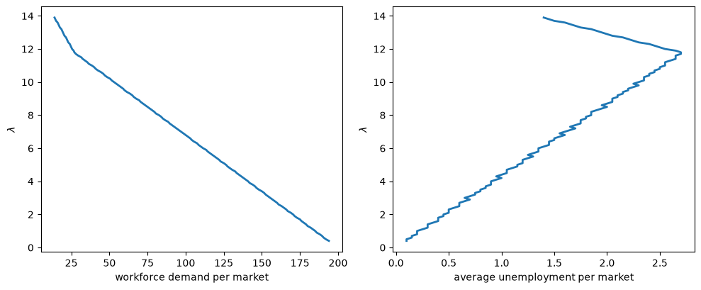
Fig. 119.6 Workforce demand and unemployment in the paper’s two-state economy#
The right panel has the shape of the bottom panels of the paper’s Figure 5: average unemployment is largest at intermediate values of \(\lambda\).
For part 2, look at the support of the invariant distribution at \(\lambda = 6\).
r_six = market_outcomes(two, 6.0)
support = np.where(r_six['ψ'].sum(axis=0) > 1e-12)[0]
print("workforce values with positive probability:", support)
print("n̄(s) =", r_six['n_bar'], "   ȳ(s) =", r_six['y_bar'])
workforce values with positive probability: [ 98 125]
n̄(s) = [ 98 140]    ȳ(s) = [ 78 125]
The two values are \(\bar n(s_{\text{low}})\) and \(\bar y(s_{\text{high}})\). To see why, follow (119.6).
In the low state the workforce is clipped into \([\bar y(s_{\text{low}}), \bar n(s_{\text{low}})]\) and in the high state into \([\bar y(s_{\text{high}}), \bar n(s_{\text{high}})]\), and at this \(\lambda\) the second interval lies entirely above the first.
So one period in the low state carries any workforce to \(\bar n(s_{\text{low}})\), one period in the high state carries it to \(\bar y(s_{\text{high}})\), and the market shuttles between the two. The same is true at every \(\lambda\) at which \(\bar n(s_{\text{low}}) < \bar y(s_{\text{high}})\), which includes the whole grid.
For part 3, unemployment is positive only in the first period of a downturn: the market enters with \(\bar y(s_{\text{high}})\) workers, demand has just fallen, and employment is \(\bar n(s_{\text{low}})\).
That event is “the state was high last period and is low now”, which has stationary probability \(\tfrac12 (1-\rho)\), so
We check the formula at every point of the grid, reading \(\rho\) from the transition matrix.
ρ_2 = two.P[0, 0]
gap2 = np.array([r['y_bar'][1] - r['n_bar'][0] for r in res2])
print(f"largest difference between formula and computation: "
      f"{np.abs(0.5*(1 - ρ_2)*gap2 - Eu2).max():.1e}")

n_lo = np.array([r['n_bar'][0] for r in res2])
print(f"unemployment per market peaks at λ = {grid2[Eu2.argmax()]:.1f}; "
      f"the low-demand market is closed for λ ≥ {grid2[n_lo == 0].min():.1f}")
largest difference between formula and computation: 4.4e-16
unemployment per market peaks at λ = 11.7; the low-demand market is closed for λ ≥ 11.8
The formula also explains the hump: average unemployment is the gap between two thresholds, multiplied by the chance of crossing it.
At high \(\lambda\) the low-demand market is closed, \(\bar n(s_{\text{low}}) = 0\), and the gap is just \(\bar y(s_{\text{high}})\), which rises as \(\lambda\) falls.
Once \(\lambda\) is low enough for the low-demand market to keep some workers, \(\bar n(s_{\text{low}})\) rises faster than \(\bar y(s_{\text{high}})\) as \(\lambda\) falls, and the gap narrows. So unemployment per market peaks where the low-demand market stops closing, as the second line of the print shows.
For part 4, the workforce is \(\bar n(s_{\text{low}})\) in half the periods and \(\bar y(s_{\text{high}})\) in the other half, so \(E[y] = \tfrac12 [\bar n(s_{\text{low}}) + \bar y(s_{\text{high}})]\) and the unemployment rate is
It rises with \(r\) toward \(1 - \rho\), which it reaches when the low-demand market closes.
For part 5, mean employment in the low state is \(\bar n(s_{\text{low}})\), and in the high state it is \(\bar y(s_{\text{high}})\) with probability \(\rho\) and \(\bar n(s_{\text{low}})\) with probability \(1 - \rho\), the first period of an upturn, so the ratio of mean employment is
Substituting \(r = (\mathcal{E} - 1 + \rho)/\rho\) into the unemployment rate of part 4 gives
which rises with \(\mathcal{E}\).
Only the construction of R changes: on the integer grid the first worker’s marginal product \(s\,\alpha\) is finite, and an empty market pays nothing. Workers are now cheap at the margin far out, so we use a larger grid, and we bracket \(\lambda^*\) around the value of search at which a market holding \(\mu\) workers would just stop attracting arrivals, \(\beta \max_s (Pv)_s\) in the notation of Exercise 119.2.
def power_R(s, y, α):
    "The marginal product s α n^(α-1) of the technology s n^α; R(s, 0) is reset to 0."
    return s[:, None]*α*np.maximum(y[None, :], 1)**(α - 1)

def solve_two_state(m, μ):
    "The equilibrium, bracketed around the value of search of an economy at rest."
    λ_rest = m.β*(m.P @ np.linalg.solve(np.eye(2) - m.β*m.P, m.R[:, μ])).max()
    r = market_outcomes(m, equilibrium_λ(m, μ, lo=0.5*λ_rest, hi=3*λ_rest))
    E_n = (r['ψ']*r['n']).sum(axis=1)/r['ψ'].sum(axis=1)   # mean employment by state
    return r, E_n

θ_k, θ_n = 0.19, 0.58
α_AV, s_AV = θ_n/(1 - θ_k), 2.12**(1/(1 - θ_k))
print(f"like AV: α = {α_AV:.3f}, s_high = {s_AV:.3f}")
economies = [('linear', two, None)]
economies += [(f'α = {α}', two_state_model(y_max=3000, R=power_R, α=α), α)
              for α in (0.4, 0.6, 0.75)]
economies += [('like AV', two_state_model(s_high=s_AV, y_max=3000, R=power_R, α=α_AV),
               α_AV)]

print(f"{'technology':>12}{'ratio of n':>12}{'ρr + 1 - ρ':>12}{'frictionless':>14}"
      f"{'u rate':>9}{'identity':>10}")
for name, m, α in economies:
    r, E_n = solve_two_state(m, μ)
    ratio, r_ratio = E_n[1]/E_n[0], r['y_bar'][1]/r['n_bar'][0]
    frictionless = (f"{(m.s[1]/m.s[0])**(1/(1 - α)):>14.2f}" if α is not None
                    else f"{'corner':>14}")
    print(f"{name:>12}{ratio:>12.2f}{ρ_2*r_ratio + 1 - ρ_2:>12.2f}{frictionless}"
          f"{100*r['unemployment']/r['workforce']:>8.2f}%"
          f"{100*(1 - ρ_2)*(ratio - 1)/(ratio - 1 + 2*ρ_2):>9.2f}%")
like AV: α = 0.716, s_high = 2.529
  technology  ratio of n  ρr + 1 - ρ  frictionless   u rate  identity
      linear        2.53        2.53        corner    4.60%     4.60%
     α = 0.4        1.63        1.63          3.17    2.60%     2.60%
     α = 0.6        2.10        2.10          5.66    3.80%     3.80%
    α = 0.75        3.29        3.29         16.00    5.60%     5.60%
     like AV        5.63        5.63         26.23    7.20%     7.20%
The identity \(\mathcal{E} = \rho r + 1 - \rho\) and the formula for the unemployment rate hold in every economy, as the columns show.
The frictionless column is (119.11) with \(\theta_k = 0\) and \(\theta_n = \alpha\): equating marginal products \(s\,\alpha\, n^{\alpha-1}\) across the two states gives \(n_{\text{high}}/n_{\text{low}} = (s_{\text{high}}/s_{\text{low}})^{1/(1-\alpha)}\).
The economy like Alvarez and Veracierto’s has the same frictionless ratio, about \(26\), as their technology with capital, because optimizing out capital turns \(z\, k^{\theta_k} n^{\theta_n}\) into a multiple of \(z^{1/(1-\theta_k)} n^{\theta_n/(1-\theta_k)}\). That labor-only form is the right comparison here, since in this model the friction falls on labor alone.
For the linear schedule the frictionless benchmark is a corner, and only just. Equating \(2(1 - n_{\text{high}}/N) = 1 - n_{\text{low}}/N\) with \(n_{\text{high}} + n_{\text{low}} = 2\mu\) gives \(n_{\text{low}} = (4\mu - N)/3\), so the low-demand market closes for every \(\mu \le N/4\), which is exactly the lecture’s \(\mu = 50\).
N = 200                                    # the capacity of the two-state economy
for μ_f in (50, 55, 60):
    n_low = max((4*μ_f - N)/3, 0.0)
    ratio = (2*μ_f - n_low)/n_low if n_low > 0 else np.inf
    print(f"μ = {μ_f}: frictionless n_low = {n_low:.1f}, ratio {ratio:.1f}")
μ = 50: frictionless n_low = 0.0, ratio inf
μ = 55: frictionless n_low = 6.7, ratio 15.5
μ = 60: frictionless n_low = 13.3, ratio 8.0
So the frictionless ratio is infinite at \(\mu = 50\) and still large just above it, against about \(2.5\) in the model.
In every economy the model responds far less than its frictionless benchmark, as a one-period moving friction should. A frictionless economy would move workers until marginal products were equal across markets; here workers move only until arriving is worth \(\lambda\), arrivals stop at \(\bar y(s_{\text{high}})\) because demand may fall back, and an upturn takes a period to be met at all.
The comparison of like with like is the last row: the technology and the shock that give Alvarez and Veracierto’s establishments an employment ratio of about \(26\) give about \(5.6\) under the one-period move of this model, although the persistence of the shock still differs from theirs.
Across the rows with \(s_{\text{high}} = 2\) the employment response rises with \(\alpha\), holding the friction fixed, and the unemployment rate rises with it. That is not a coincidence, and it is this lecture’s finding rather than Baley, Ljungqvist and Sargent’s.
Unemployment in this model is the time workers spend moving, and the more there is to gain by moving, the more of them move: holding the friction fixed, an economy with higher returns to labor mobility shows more reallocation and records the unemployment that goes with it.
Exercise 119.4
This exercise asks what the model’s directed search is doing.
Alvarez and Veracierto [1999] replace it with undirected search: a searcher cannot choose where to go, and every market receives the same inflow \(U\), which is the economy’s unemployment per market.
Show that under undirected search the \(\min\) disappears from (119.2), and say which economic condition it was enforcing.
Write down the transition law for a market’s workforce, and show that at any stationary distribution the inflow \(U\) equals the average outflow. Does the same identity hold under directed search?
Under directed search, (119.8) pins down \(\lambda\). Under undirected search, what condition must \(\lambda\) satisfy instead? Count the unknowns and the conditions of an equilibrium with a fixed workforce \(\mu\) per market.
Compute the undirected equilibrium of the lecture’s economy, \(\mu/N = 1/4\). An integer inflow into markets of capacity \(N = 200\) is too coarse, so count workers in tenths: use \(N = 2000\) and a grid up to \(2600\), which is the lecture’s economy on a ten times finer workforce grid. For inflows \(U = 1, 3, 5, 7, 9\) and \(10\), find the values of \(\lambda\) that satisfy the consistency condition of part 3 and the mean workforce that each serves, and plot the mean workforce against \(U\). How many equilibria does an economy with a given \(\mu\) have? Compare \(\lambda\) and the unemployment rate at \(\mu/N = 1/4\) with directed search on the same grid.
Explain why undirected search lowers the value of search here, and why it also lowers unemployment.
Solution
For part 1, the \(\min\) in (119.2) is the restriction, imposed by competition among searchers, that the continuation value in a market cannot exceed \(\lambda\). Take away their ability to choose where to go and nothing enforces it.
A worker who stays simply collects the wage and the continuation value his own market happens to deliver,
and the continuation can be worth more or less than \(\lambda\), because nobody can act on the difference.
For part 2, employment is still \(n(s,y) = \min\{\bar n(s), y\}\), those not employed leave, and the inflow is the same everywhere, so
At a stationary distribution \(E[y'] = E[y]\), so averaging across markets gives
the inflow equals the average outflow.
That is an accounting identity, and it holds under directed search too: at the stationary distribution of (119.6), the workers arriving in markets that fill up equal the workers leaving markets that shed, at every value of \(\lambda\) and not only at \(\lambda^*\).
print(f"{'λ':>8}{'E[y]':>9}{'outflow':>10}{'inflow':>9}")
y = model.y[None, :]
for λ in (4.0, 7.1, 10.0):
    r = market_outcomes(model, λ)
    y_next = np.clip(y, r['y_bar'][:, None], r['n_bar'][:, None])
    print(f"{λ:>8.3f}{r['workforce']:>9.2f}"
          f"{(r['ψ']*np.maximum(y - y_next, 0)).sum():>10.4f}"
          f"{(r['ψ']*np.maximum(y_next - y, 0)).sum():>9.4f}")
       λ     E[y]   outflow   inflow
   4.000   114.97    0.6512   0.6512
   7.100    49.92    1.0647   1.0647
  10.000     8.71    0.4841   0.4841
So the identity cannot be what distinguishes the two models; what does is how \(\lambda\) is determined.
For part 3, a searcher under undirected search lands in a market drawn at random from the invariant distribution, so the value of search must satisfy
the discounted value of landing in a randomly drawn market, a market-weighted average.
An equilibrium with a fixed population therefore has two unknowns, \(\lambda\) and \(U\), and two conditions, \(\mu = \sum_{s,y} \psi(s,y)\, y\) and the condition above.
Under directed search the \(\min\) makes every market that receives workers worth exactly \(\lambda\), so \(\lambda\) needs no separate consistency condition, and \(\mu\) pins it down alone through a schedule that slopes down. Here \(\lambda\) needs a condition of its own, and nothing makes that condition monotone in \(\lambda\).
For part 4, a market’s employment threshold is the largest workforce at which staying is still worth \(\lambda\), given that next period’s workforce will be \(n(s, y) + U\).
The invariant distribution is unique, because a market that passes through the worst demand state ends up holding \(\bar n(s_1) + U\) workers from anywhere, so we find it by iterating on it.
def undirected_market(model, λ, U, tol=1e-10, max_iter=100_000):
    """A market that receives U searchers every period, whether it wants them or not.
    Returns the implied value of search, the mean workforce, and n̄(s)."""
    P, R, β, y = model.P, model.R, model.β, model.y
    n_s, n_y = R.shape
    up = np.minimum(y + U, y[-1])                  # next workforce if nobody leaves
    v = np.full(R.shape, λ)
    for _ in range(max_iter):
        v_new = np.maximum(λ, R + β*(P @ v)[:, up])
        if np.max(np.abs(v_new - v)) < tol:
            break
        v = v_new
    else:
        raise RuntimeError(f"the value function did not converge at λ = {λ}")
    n_bar = last_at_least(R + β*(P @ v_new)[:, up], λ)
    if n_bar.max() + U > y[-1]:
        raise GridTooSmall(f"n̄ + U passes the top of the grid at λ = {λ}")
    # iterate on the distribution of (s, y) under y' = min(y, n̄(s)) + U
    to = (np.arange(n_s)[:, None]*n_y + np.minimum(y[None, :], n_bar[:, None]) + U).ravel()
    ψ = np.full(n_s*n_y, 1/(n_s*n_y))
    for _ in range(max_iter):
        ψ_new = (P.T @ np.bincount(to, weights=ψ, minlength=n_s*n_y).reshape(n_s, n_y)).ravel()
        if np.abs(ψ_new - ψ).sum() < tol:
            break
        ψ = ψ_new
    else:
        raise RuntimeError(f"the distribution did not converge at λ = {λ}")
    ψ = ψ_new.reshape(n_s, n_y)
    return β*(ψ*v_new).sum(), (ψ*y).sum(), n_bar
The gap between the implied value of search and \(\lambda\) turns out to be positive between two roots and negative outside them, so for each inflow we look for one root on each side of a value where it is positive.
On this grid the directed-search \(\lambda^*\) is such a value at every inflow that has roots, and brentq from SciPy stops with an error if a bracket fails.
def consistent_λs(model, U, λ_mid, lo=0.1, hi=12.0):
    "The roots of λ = β Σ ψ v below and above λ_mid, with the mean workforce of each."
    gap = lambda λ: undirected_market(model, λ, U)[0] - λ
    roots = (brentq(gap, lo, λ_mid, xtol=2e-3), brentq(gap, λ_mid, hi, xtol=2e-3))
    return [(λ, undirected_market(model, λ, U)[1]) for λ in roots]

N_fine = 2000                            # the lecture's economy, in tenths of a worker
m_fine = create_model(N=N_fine, y_max=13*N_fine//10)
λ_dir = equilibrium_λ(m_fine, N_fine//4)
r_dir = market_outcomes(m_fine, λ_dir)

locus = {U: consistent_λs(m_fine, U, λ_dir) for U in (1, 3, 5, 7, 9)}
gaps_10 = [undirected_market(m_fine, λ, 10)[0] - λ for λ in np.arange(6.0, 8.6, 0.5)]
print(f"at U = 10 the largest gap on a grid of λ is {max(gaps_10):.4f}")
at U = 10 the largest gap on a grid of λ is -0.0418
Each of these inflows has two solutions, and each serves its own population; at \(U = 10\) there are none.
Us = np.array(list(locus))
scale = 200/N_fine                       # back to the lecture's units
fig, ax = plt.subplots(figsize=(7, 4))
for k, label in ((0, r'crowded: lower $\lambda$'), (1, r'sparse: higher $\lambda$')):
    ax.plot(scale*Us, [scale*locus[U][k][1] for U in Us], 'o-', lw=2, label=label)
ax.axhline(50, color='k', lw=0.8, ls='--', label=r'$\mu = 50$')
ax.set_xlabel('inflow $U$ per market of capacity 200')
ax.set_ylabel(r'workforce per market $\mu$')
ax.legend()
plt.tight_layout()
plt.show()
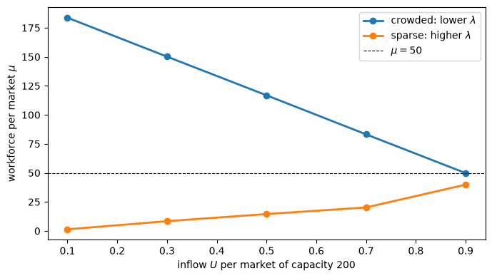
Fig. 119.7 Undirected search, the populations served by the solutions at each inflow#
At a given inflow the two solutions belong to different populations, a crowded economy with a low value of search and a sparse one with a high value. Along each branch the population moves monotonically with the inflow, the two branches meet in a fold between \(U = 9\) and \(U = 10\), and their ranges of \(\mu\) do not overlap.
So in this calibration each population has exactly one undirected equilibrium \((\lambda, U)\), and the inflow it needs rises with \(\mu\) up to the fold and falls beyond it.
The fold also explains why \(N = 200\) will not do: the largest equilibrium inflow is a little below one worker per market of capacity 200, so even \(U = 1\) on that grid is past it. The lecture’s economy is the point nearest \(\mu = 50\).
U_eq, k_eq = min(((U, k) for U in locus for k in (0, 1)),
                 key=lambda Uk: abs(locus[Uk[0]][Uk[1]][1] - N_fine//4))
λ_und, y_und = locus[U_eq][k_eq]
print(f"undirected: U = {U_eq}, λ = {λ_und:.3f}, workforce {scale*y_und:.2f}, "
      f"unemployment rate {100*U_eq/y_und:.2f}%")
print(f"directed:   λ* = {λ_dir:.3f}, workforce {scale*r_dir['workforce']:.2f}, "
      f"unemployment rate {100*r_dir['unemployment']/r_dir['workforce']:.2f}%")
undirected: U = 9, λ = 6.906, workforce 49.80, unemployment rate 1.81%
directed:   λ* = 7.126, workforce 50.00, unemployment rate 2.13%
It lies on the crowded branch, close to the fold, and undirected search gives it a lower value of search and a lower unemployment rate than directed search does.
For part 5, compare the employment thresholds.
n_bar_und = undirected_market(m_fine, λ_und, U_eq)[2]
n_bar_low, _ = thresholds(m_fine, worker_value(m_fine, λ_und)[0], λ_und)
print("n̄(s), undirected:                       ", n_bar_und)
print("n̄(s), directed, at its own λ*:          ", r_dir['n_bar'])
print("n̄(s), directed, at the undirected λ:    ", n_bar_low)
n̄(s), undirected:                        [  77  297  518  732  933 1113 1269]
n̄(s), directed, at its own λ*:           [   0  161  449  694  905 1087 1246]
n̄(s), directed, at the undirected λ:     [   0  218  496  734  939 1116 1269]
Undirected search lowers the value of search because searchers can no longer avoid markets that do not want them: under directed search every searcher goes where arriving is worth \(\lambda\), while here many land in markets that are shedding workers or soon will.
With a lower value of search, workers whose market’s demand has fallen are slower to leave: the employment thresholds are higher in every demand state, and outside the lowest demand states most of the difference is what directed search itself would give at the same lower \(\lambda\), as the last line shows. So markets keep more of their workers, and the economy holds its population with a smaller flow of searchers, which is its unemployment.
Note that for a given inflow, the map from a perceived \(\lambda\) to the implied value \(\beta \sum \psi v\) is a genuine map from a perceived to an actual value of search, unlike the tâtonnement of Learning the value of search.
Exercise 119.5
The model has no aggregate shocks, but Lucas and Prescott open their concluding remarks by arguing that its mechanism “is consistent with the now familiar account of the observed Phillips curve in terms of expectations”:
an unanticipated change in aggregate demand (a change in \(E(s'|s)\)) will move unemployment and wage changes in opposite directions.
Check this at the equilibrium of the lecture, starting from the invariant distribution at \(\lambda^*\), which describes the economy last period.
This period, a share of markets chosen at random draws a demand state one notch lower than the law of motion that everyone knows would give it, and the rest draw as usual; the share is chosen so that mean \(\log s\) falls by \(\Delta\).
Nobody anticipated it, so the thresholds \(\bar n(s)\) and \(\bar y(s)\) stay as they were, and \(\lambda\) stays at \(\lambda^*\).
Compute this period’s unemployment rate and mean wage for \(\Delta = 0.01, 0.02, 0.04\), and for rises in mean \(\log s\) of the same sizes.
Plot the unemployment rate against the percentage change in the mean wage. Explain the shape.
Lucas and Prescott add that if such changes “were a recurrent event, as they are in reality, this fact would become incorporated into the maximum problem facing workers”. What would change in the calculation?
Solution
The surprise changes only the transition matrix that applies this period, so we carry last period’s markets forward with the thresholds they already have and draw this period’s demand from the altered matrix.
def demand_surprise(model, r, Δ):
    """This period's unemployment rate and mean wage when mean log demand moves by Δ:
    a share |Δ|/notch of markets draws a state one notch away from the usual draw."""
    n_s, y = len(model.s), model.y
    notch = np.log(model.s[1]/model.s[0])
    step = int(np.sign(Δ))
    move = np.zeros((n_s, n_s))                       # shift a state, within the grid
    move[np.arange(n_s), np.clip(np.arange(n_s) + step, 0, n_s - 1)] = 1
    P_now = (1 - abs(Δ)/notch)*model.P + abs(Δ)/notch*(model.P @ move)
    y_carried = np.clip(y[None, :], r['y_bar'][:, None], r['n_bar'][:, None])
    ψ_now = sum(np.outer(P_now[i], np.bincount(y_carried[i], weights=r['ψ'][i],
                                               minlength=len(y)))
                for i in range(n_s))
    n, w = r['n'], r['w']
    rate = (ψ_now*(y[None, :] - n)).sum()/(ψ_now*y[None, :]).sum()
    return rate, (ψ_now*n*w).sum()/(ψ_now*n).sum()

r_star = market_outcomes(model, equilibrium_λ(model, μ))
base_rate, base_wage = demand_surprise(model, r_star, 0.0)
print(f"no surprise: unemployment rate {100*base_rate:.2f}%, mean wage {base_wage:.4f}")
print(f"{'Δ':>7}{'u rate':>9}{'wage change':>13}{'per unit of Δ':>15}")
points = [(100*base_rate, 0.0)]
for Δ in (-0.04, -0.02, -0.01, 0.01, 0.02, 0.04):
    rate, mean_wage = demand_surprise(model, r_star, Δ)
    change = 100*(mean_wage/base_wage - 1)
    points.append((100*rate, change))
    print(f"{Δ:>7}{100*rate:>8.2f}%{change:>12.2f}%{change/(100*Δ):>15.2f}")
no surprise: unemployment rate 2.13%, mean wage 0.7742
      Δ   u rate  wage change  per unit of Δ
  -0.04    5.65%       -1.97%           0.49
  -0.02    3.89%       -0.97%           0.48
  -0.01    3.01%       -0.48%           0.48
   0.01    2.04%        1.03%           1.03
   0.02    1.94%        2.06%           1.03
   0.04    1.75%        4.11%           1.03
The no-surprise line reproduces the equilibrium, as it should.
u_pts, w_pts = np.array(sorted(points)).T
fig, ax = plt.subplots(figsize=(6.5, 4))
ax.plot(u_pts, w_pts, 'o-', lw=2)
ax.axhline(0, color='k', lw=0.8)
ax.set_xlabel('unemployment rate (%)')
ax.set_ylabel('change in the mean wage (%)')
plt.tight_layout()
plt.show()
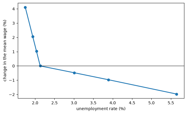
Fig. 119.8 An unanticipated shift in demand moves unemployment and wages in opposite directions#
Unemployment and wages move in opposite directions, as Lucas and Prescott say, and the points trace out a downward-sloping curve with a kink at the equilibrium: a Phillips curve.
A surprise fall in demand pushes some markets below their employment thresholds, and they shed workers, so unemployment rises a lot. Wages fall, but by less than demand, because the markets that shed cut employment, which raises the marginal product of those who stay.
A surprise rise in demand can lower unemployment only by preventing separations that would have happened anyway, and there are few of those, while every market’s wage rises with its demand, about one for one, and no new workers can arrive within the period to hold it down.
So the curve is steep where unemployment is low and flat where it is high.
The signs and the kink do not depend on the grid, but the size of the unemployment response does: a notch is about a fifth in \(\log s\) on the seven-state chain, so a given fall in mean log demand is concentrated on few markets, each hit hard, and with finer chains the same fall raises unemployment by less.
For part 3, the calculation holds the thresholds and \(\lambda\) fixed because nobody expected the shift. If such shifts recurred, workers would build them into the transition law they use, the Bellman equation would change, and so would \(\bar n\), \(\bar y\) and \(\lambda^*\); Lucas and Prescott leave that “nontrivial development for future research”.
The Rise and Fall of U.S. Inflation follows the expectational account of the Phillips curve, and the natural-rate hypothesis behind it, into the data.
Exercise 119.6
Efficiency proves that the equilibrium solves the planner’s problem (119.10). Check it numerically, and see what it does and does not imply.
Solve (119.10) at \(\lambda^*\) by value function iteration, choosing \(y'\) on the whole grid, and verify that \(W(s, y) - W(s, y-1) = v(s, y)\) and that the planner’s choice of \(y'\) is (119.6).
Now let moving use up resources: each worker who leaves costs \(c = 2\). Show that the equilibrium of Exercise 119.2 is the allocation of a planner who faces that cost, credited \(\lambda - c\) for each worker released and charged \(\lambda\) for each worker brought in. What does that imply about the lower surplus in Exercise 119.2?
Compare steady-state surplus per worker at the equilibrium with two alternatives that keep \(\mu = 50\): a small subsidy to moving, \(c = -0.1\) and \(c = -0.2\), and the thresholds that a more patient planner would choose, with \(\beta' = 0.95\) and \(0.99\) and \(\lambda\) chosen to keep \(\mu\) workers per market. Does the equilibrium maximize steady-state surplus? Reconcile the answer with Efficiency.
Solution
For part 1, planner_value solves (119.10), with the release credit lowered to \(\lambda - c\) for part 2. The flow term does not depend on \(W\), so we compute it once.
def planner_value(model, λ, c=0.0, tol=1e-10, max_iter=10_000):
    """W(s, y) = max over y' of Φ(s, min(y, y')) + credit for releases - charge for
    arrivals + β E W(s', y'), with releases credited at λ - c and arrivals charged λ."""
    P, R, β, y = model.P, model.R, model.β, model.y
    Φ = np.cumsum(R, axis=1)
    moved = y[:, None] - y[None, :]                  # workers released, for each (y, y')
    flow = (Φ[:, np.minimum(y[:, None], y[None, :])]
            + np.where(moved > 0, (λ - c)*moved, λ*moved))
    W = np.zeros(R.shape)
    for _ in range(max_iter):
        value = flow + β*(P @ W)[:, None, :]
        W_new = value.max(axis=2)
        if np.max(np.abs(W_new - W)) < tol:
            return W_new, y[value.argmax(axis=2)]
        W = W_new
    raise RuntimeError(f"no convergence in {max_iter} iterations at λ = {λ}")

def check_planner(model, λ, c=0.0):
    "Compare the planner's marginal values and policy with the equilibrium."
    r = market_outcomes(model, λ, c)
    W, y_choice = planner_value(model, λ, c)
    law = np.clip(model.y[None, :], r['y_bar'][:, None], r['n_bar'][:, None])
    print(f"c = {c}, λ = {λ:.3f}: largest |ΔW - v| = "
          f"{np.abs(np.diff(W, axis=1) - r['v'][:, 1:]).max():.1e}, "
          f"policy equals the transition law: {np.array_equal(y_choice, law)}")

λ_0 = equilibrium_λ(model, μ)
check_planner(model, λ_0)
c = 0.0, λ = 7.096: largest |ΔW - v| = 3.8e-11, policy equals the transition law: True
For part 2, the same check with the resource cost.
λ_2 = equilibrium_λ(model, μ, 2.0, lo=λ_0)
check_planner(model, λ_2, 2.0)
c = 2.0, λ = 8.262: largest |ΔW - v| = 6.9e-11, policy equals the transition law: True
With a resource cost, the equilibrium is the planner’s allocation for the costlier technology of moving: the argument of Efficiency goes through with the release credit \(\lambda - c\), and the resource cost enters surplus.
So the lower surplus that Exercise 119.2 finds with a resource cost is the price of a worse technology, and the equilibrium makes the best of it. A rebated tax changes decisions in exactly the same way but uses up nothing, so the technology is the laissez-faire one, whose planner chooses the laissez-faire allocation, and the taxed equilibrium is distorted: its lower surplus is an efficiency loss.
For part 3, a subsidy is a negative \(c\), and a more patient planner’s thresholds come from the worker’s problem with \(\beta'\) in place of \(\beta\).
def steady_state(model, policy, λ):
    """Steady-state surplus, unemployment and workforce per market of model when its
    markets follow the thresholds that the worker's problem in policy gives at λ."""
    n_bar, y_bar = thresholds(policy, worker_value(policy, λ)[0], λ)
    ψ = stationary_distribution(model, n_bar, y_bar)
    y = model.y[None, :]
    n = np.minimum(y, n_bar[:, None])
    return ((ψ*np.take_along_axis(np.cumsum(model.R, axis=1), n, axis=1)).sum(),
            (ψ*(y - n)).sum(), (ψ*y).sum())

r_0 = market_outcomes(model, λ_0)
print(f"{'':>24}{'surplus per worker':>20}{'u rate':>9}{'workforce':>11}")
print(f"{'equilibrium':>24}{r_0['surplus']/r_0['workforce']:>20.5f}"
      f"{100*r_0['unemployment']/r_0['workforce']:>8.2f}%{r_0['workforce']:>11.2f}")
for c in (-0.1, -0.2):
    r = market_outcomes(model, equilibrium_λ(model, μ, c, lo=2.0, hi=λ_0), c)
    print(f"{f'subsidy {-c}':>24}{r['surplus']/r['workforce']:>20.5f}"
          f"{100*r['unemployment']/r['workforce']:>8.2f}%{r['workforce']:>11.2f}")
for β_p in (0.95, 0.99):
    patient = model._replace(β=β_p)
    λ_p = bisect(lambda λ: steady_state(model, patient, λ)[2] <= μ, 0.01, 2000.0)
    s_p, u_p, y_p = steady_state(model, patient, λ_p)
    print(f"{f'patient planner, β = {β_p}':>24}{s_p/y_p:>20.5f}"
          f"{100*u_p/y_p:>8.2f}%{y_p:>11.2f}")
                          surplus per worker   u rate  workforce
             equilibrium             0.93521    2.13%      49.94
             subsidy 0.1             0.93549    2.37%      49.99
             subsidy 0.2             0.93571    2.60%      49.94
patient planner, β = 0.95             0.93561    2.35%      49.97
patient planner, β = 0.99             0.93565    2.42%      50.00
Both alternatives raise steady-state surplus per worker above its equilibrium level, and both do it with more reallocation and more unemployment. So the equilibrium does not maximize steady-state surplus, and Efficiency never said it did.
The theorem compares present values starting from the equilibrium’s own distribution, and a move to one of these steady states would cost surplus along the way: more workers in transit means a period of their output lost now, for gains that come later and are discounted.
A planner who discounted at \(\beta' > \beta\) would value those later gains more, which is why its thresholds move more workers; in the limit of no discounting it would maximize steady-state surplus, the analogue of the golden rule, and the equilibrium is the analogue of the modified golden rule.
The steady-state comparison in Exercise 119.2 points the same way as the theorem for a large cost, but that is not something the theorem implies: a small subsidy, which also moves the economy away from the planner’s allocation, raises steady-state surplus.